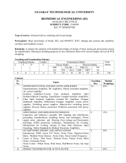
Magnetic Resonance Imaging 32 (2014) 702–720 Contents lists available at ScienceDirect Magnetic Resonance Imaging journal homepage: www.mrijournal.com Generalized total variation-based MRI Rician denoising model with spatially adaptive regularization parameters Ryan Wen Liu a, b, Lin Shi b, c,⁎, Wenhua Huang d,⁎⁎, Jing Xu d, Simon Chun Ho Yu a, Defeng Wang a, b, e, f a Department of Imaging and Interventional Radiology, The Chinese University of Hong Kong, Shatin, New Territories, Hong Kong SAR, P.R. China Research Center for Medical Image Computing, The Chinese University of Hong Kong Shatin, New Territories, Hong Kong SAR, P.R. China Department of Medicine and Therapeutics, The Chinese University of Hong Kong, Shatin, New Territories, Hong Kong SAR, P.R. China d Institute of Clinical Anatomy, Southern Medical University, Guangzhou, Guangdong, P.R. China e CUHK Shenzhen Research Institute, Shenzhen, Guangdong, P.R. China f Department of Biomedical Engineering and Shun Hing Institute of Advanced Engineering, The Chinese University of Hong Kong, Shatin, New Territories, Hong Kong SAR, P.R. China b c a r t i c l e i n f o Article history: Received 28 June 2013 Revised 13 January 2014 Accepted 7 March 2014 Keywords: Total variation Magnetic resonance imaging (MRI) Diffusion tensor MRI (DT-MRI) Image denoising Hyper-Laplacian prior Rician distribution a b s t r a c t Magnetic resonance imaging (MRI) is an outstanding medical imaging modality but the quality often suffers from noise pollution during image acquisition and transmission. The purpose of this study is to enhance image quality using feature-preserving denoising method. In current literature, most existing MRI denoising methods did not simultaneously take the global image prior and local image features into account. The denoising method proposed in this paper is implemented based on an assumption of spatially varying Rician noise map. A two-step wavelet-domain estimation method is developed to extract the noise map. Following a Bayesian modeling approach, a generalized total variation-based MRI denoising model is proposed based on global hyper-Laplacian prior and Rician noise assumption. The proposed model has the properties of backward diffusion in local normal directions and forward diffusion in local tangent directions. To further improve the denoising performance, a local variance estimator-based method is introduced to calculate the spatially adaptive regularization parameters related to local image features and spatially varying noise map. The main beneﬁt of the proposed method is that it takes full advantage of the global MR image prior and local image features. Numerous experiments have been conducted on both synthetic and real MR data sets to compare our proposed model with some state-of-the-art denoising methods. The experimental results have demonstrated the superior performance of our proposed model in terms of quantitative and qualitative image quality evaluations. © 2014 Elsevier Inc. All rights reserved. 1. Introduction 1.1. Background and related work Magnetic resonance imaging (MRI) is an outstanding medical imaging modality but often suffers from noise pollution during image acquisition and transmission. For single-coil MR acquisitions, the magnitude MR images are usually modeled using a Rician distribution. If multiple-coil acquisitions and no subsampling of the k-space raw data are considered, the magnitude data will follow a non-central Chi (nc-χ) distribution [1–3]. MRI denoising has attracted tremendous attentions of researchers in the ﬁeld of biomedical imaging. Compared with non-medical imaging applications, ⁎ Correspondence to: Lin Shi, Department of Medicine and Therapeutics, The Chinese University of Hong Kong, Shatin, New Territories, Hong Kong SAR, P.R. China. Tel.: +852 26322975; fax: +852 26487269. ⁎⁎ Correspondence to: Wenhua Huang, Institute of Clinical Anatomy, Southern Medical University, Guangzhou, Guangdong, P.R. China. Tel.: +86 20 61648183. E-mail addresses: [email protected] (L. Shi), hwh@ﬁmmu.com (W. Huang). http://dx.doi.org/10.1016/j.mri.2014.03.004 0730-725X/© 2014 Elsevier Inc. All rights reserved. MRI denoising methods should put more emphasis on preservation of ﬁne structures during noise reduction. In clinical settings, the ﬁne structures contain important medical information, which could assist physicians with accurate diagnosis. There are a variety of study methods that have been developed for MRI denoising. Henkelman [4] presented the ﬁrst attempt to estimate the noiseless magnitude MR image from its noisy version. Recent methods on MRI denoising have employed nonparametric statistical techniques. For example, Awate and Whitaker [5] proposed a novel MRI denoising method with nonparametric neighborhood statistics. They also introduced a feature-preserving denoising approach by inferring uncorrupted-signal Markov statistics as a prior under an empirical Bayesian framework [6]. More recently, López-Rubio and Florentín-Núñez [7] considered a nonparametric regression method depending on a zeroth order three-dimensional (3D) kernel regression, which computed a weighted average of pixels over a regression window. A novel 3D image denoising procedure was developed using local smoothing and nonparametric regression [8]. This method could preserve edges and major edge structures in the restored MR images. R.W. Liu et al. / Magnetic Resonance Imaging 32 (2014) 702–720 Wavelet transform-based approaches have also been considered in the literature [9,10]. The image in wavelet domain is decomposed into a set of multiresolutional wavelet coefﬁcients. The detail coefﬁcients are processed with hard or soft thresholding at some particular levels to effectively remove noise from an image [11]. Wood and Johnson [12] have used wavelet packets for Rician noise reduction in low signal-to-noise ratio (SNR) MR images. Recently, a hybrid denoising method which combined the 3D optimized blockwise nonlocal-means (NLM) ﬁlter [13] with discrete wavelet transform was proposed based on a multiresolution approach [14]. Anand and Sahambi [15] presented a wavelet-based bilateral ﬁltering scheme which has achieved remarkable denoising performance. Besides, many other transforms have also been successfully applied to reduce Rician noise. For instance, Manjón et al. [16] introduced a new noise reduction method by using an overcomplete local principal component analysis (PCA)-based decomposition. Two-dimensional (2D) principal component decomposition and Haar transformation were incorporated into the structure-adaptive sparse denoising scheme [17]. The discrete cosine transform (DCT)-based MRI denoising methods have also attracted much attention in recent years [18,19]. Other denoising methods have been presented based on partial differential equations (PDE). The anisotropic diffusion (AD) ﬁlter was ﬁrst introduced by Gerig et al. [20] to MRI in 1992. By Basu et al. [21] the Rician noise model was incorporated into the Perona-Malik ﬁlter [22] for denoising of diffusion tensor MRI (DT-MRI) in the maximum a posteriori (MAP) framework. However, the AD-based methods were highly dependent on some parameters, such as edge enhancement parameter, conductance parameter and iteration stopping time [23]. To overcome this disadvantage, Tong et al. [24] presented an automatic parameter selection scheme for AD ﬁlter. In 2009, Krissian and AjaFernández [25] introduced an extension of the speckle reducing anisotropic diffusion (SRAD) [26] to remove Rician noise. More recently, Golshan et al. [27] proposed an effective denoising method based on SNR-adapted nonlocal linear minimum mean square error (SNLMMSE). A recursive version (RSNLMMSE) of SNLMMSE was also addressed to further enhance denoising performance. Following Buades et al. [28], the NLM-based denoising methods have received considerable attention during recent years. In the NLM-based methods, each noiseless pixel value is estimated by the weighted average of pixels with related surrounding neighborhoods [29]. But the methods may result in ineffective MRI denoising, because they generate satisfactory results only under the assumption of Gaussian random noise. Based on the second-order moment of a Rician distribution, the unbiased NLM (UNLM) was extended to reduce Rician-distributed noise present in low-SNR MRI [30,31]. Furthermore, Coupé et al. [13] proposed an effective denoising method based on a 3D optimized blockwise version of the NLM. From a statistical point of view, nonlocal maximum likelihood (NLML) estimation methods have been considered [32,33]. More recently, Manjón et al. [18] presented two novel 3D MRI denoising techniques based on sparseness and self-similarity, i.e., oracle-based DCT ﬁlter (ODCT3D) and preﬁltered rotationally invariant NLM ﬁlter (PRI-NLM3D). MR images in practice tend to be inﬂuenced by spatially varying Rician noise [34], the above-mentioned methods easily lead to unsatisfactory denoising results. To overcome this limitation, Manjón et al. [35] have developed an adaptive NLM-based method to deal with the inhomogeneous distribution of noise. Apart from the aforementioned methods, several denoising methods have been considered based on total variation (TV) regularizer. The TV-based method, ﬁrst proposed by Rudin et al. [36], is capable of preserving edges and removing image noise in homogeneous regions. Drapaca [37] has investigated the effects of regularization parameters on TV-based MRI denoising results. Wang and Zhou [38] proposed a hybrid MRI denoising method by combining the TV scheme with wavelet transform. However, these 703 TV-based models were presented based on the noise assumption of Gaussian distribution, which was different from the Rician distribution present in degraded MR images. Following a Bayesian modeling approach, the Rician-distributed-based TV models have been considered for MRI denoising [39,40]. More recently, Riciandistributed-based second-order total generalized variation (TGV) model and its modiﬁed versions have also been proposed to enhance medical image quality [41,42]. We mainly focus on the TV-based MRI denoising method in this paper. 1.2. Motivation and contributions It is well known that the regularization parameter plays a critical role in TV-based noise reduction. To achieve good denoising results, the parameter should be calculated adaptively according to local image features. In current literature, the optimal selection of regularization parameter has attracted increasing amounts of attention for TV-based additive/multiplicative noise removal. As discussed in Refs. [43,44], the regularization parameter was inversely proportional to the scale of image feature. Thus the parameters localized at image features of different scales should be selected differently. In particular, the parameters are large in detail regions with small-scale features and small in homogeneous regions with large-scale features. Gilboa et al. [45] developed an adaptive texture-preserving denoising method which controlled the level of denoising by computing the spatially varying constrains based on local variance measures. Dong et al. [44] proposed a multi-scale TV-based image restoration model with an automatic selection of spatially adaptive regularization parameter scheme to enhance image details while removing noise in homogeneous regions. These TV-based methods have gained a lot of attention due to their ability to effectively reduce additive Gaussian noise. To remove multiplicative gamma and Poisson noise, Li et al. [46,47] and Chen and Cheng [48] have also developed local feature-based methods to estimate the adaptive regularization parameters to generate good denoising results. However, the magnitude MRI signal in practice is corrupted by a Rician or nc-χ noise, not a Gaussian, gamma or Poisson one. Thus the aforementioned TV-based methods are unable to effectively reduce the noise present in magnitude MR images. There is a huge potential to develop an automatic method to select the spatially adaptive regularization parameter scheme for TV-based MRI denoising models [39,40]. On the other hand, most existing denoising methods are based on an assumption of uniform distribution of noise standard deviation (NSD) across an image. In contrast, our proposed denoising method will be implemented based on a more natural assumption of spatially varying Rician noise map (i.e., spatially varying distributed NSD). In this paper, a generalized total variation (GTV)-based MRI Rician denoising method is proposed based on global hyper-Laplacian image prior and Rician noise assumption. In what follows, a local variance estimatorbased method is developed to calculate the spatially adaptive regularization parameters related to local image features and spatially varying noise map. Our proposed MRI denoising framework signiﬁcantly differs from previous works in the following aspects: 1. The denoising method proposed in this paper is implemented based on an assumption of spatially varying Rician noise map. Before doing noise reduction, a two-step wavelet-domain estimation method is introduced to extract the spatially varying noise map for each voxel individually. 2. Following a Bayesian modeling approach, a GTV-based MRI denoising model is proposed based on global hyper-Laplacian image prior and Rician noise assumption. The proposed model has the properties of backward diffusion in local normal directions and forward diffusion in local tangent directions to perform feature-preserving denoising. 704 R.W. Liu et al. / Magnetic Resonance Imaging 32 (2014) 702–720 Fig. 1. Characteristics of Rician noise in MRI. From top-left to top-right: a 2D T1-weighted MR image corrupted by 15% of Rician noise and a mask image separating the background, low-SNR and high-SNR regions. As shown, the Rician noise tends to be Gaussian distributed when SNR is high (bottom-left) and Rayleigh distributed when SNR closes to zero (bottom-right). In low-SNR regions, the Rician noise tends to be neither Gaussian nor Rayleigh distributed (bottom-middle). 3. To further improve the denoising performance, a local variance estimator-based method is introduced to calculate the spatially adaptive regularization parameters according to local image features and spatially varying noise map. In particular, the large regularization parameters in texture regions result in ﬁne detail preservation; whereas small ones in homogeneous regions perform well in noise reduction. and estimation of spatially varying noise map in MRI. In Section 3, we present the GTV-based MRI Rician denoising model with spatially adaptive regularization parameters. Numerous experiments on both synthetic and real MR data sets are performed in Section 4. Finally we conclude this paper by summarizing our contributions and discussing the future work in Section 5. 2. Noise estimation in magnitude MR images The main beneﬁt of our proposed method is that it takes full advantage of the global MR image prior and local image features. Thus it can effectively reduce noise levels while preserving edges and ﬁne scale details in practice. 1.3. Organization The remainder of this paper is organized into several sections. Section 2 brieﬂy explains the Rician noise distribution 2.1. Noise characteristics in MRI In MRI the measured signal magnitude consists of real and imaginary parts. If both real and imaginary parts are corrupted by the zero-mean uncorrelated Gaussian noise with equal variance, noise in magnitude MRI data can no longer be modeled by the Gaussian distribution via the complex Fourier transformation [34]. As mentioned in Introduction, the magnitude Fig. 2. Left: graphical representation of the function F(θ) with different magnitudes of 〈M〉/σ. Right: the correction factor ξ(θ) as a function of SNR = θ. R.W. Liu et al. / Magnetic Resonance Imaging 32 (2014) 702–720 signal from a multiple-coil MR acquisition system follows a nc-χ distribution [49] ! n−1 2 2 M M M þ A MA In−1 pðMjA; σ Þ ¼ 2 exp − ; ð1Þ 2 2 A σ σ 2σ where M is the value in the magnitude image, A is the amplitude of the noiseless signal, σ 2 denotes the variance of Gaussian noise in complex domain, n is the number of channels used for parallel data acquisition, and In − 1(⋅) represents the (n − 1)th-order modiﬁed Bessel function of the ﬁrst kind. Without loss of generality, we only consider the case of n = 1 in this paper, then (1) reduces to the Rician distribution [50], i.e., ! 2 2 M M þ A MA pðMjA; σ Þ ¼ 2 exp − : ð2Þ I0 2σ 2 σ σ2 Rician distribution is essentially a special case of the nc-χ distribution. In this paper, let us deﬁne SNR as A/σ. Once the noiseless signal A tends to zero in image background (i.e., SNR → 0), the Rician distribution (2) can simplify to a Rayleigh distribution. In contrast, the noise distribution in high-SNR regions can be approximated by a Gaussian distribution [51]. Fig. 1 shows the characteristics of Rician noise in MRI. In low-SNR regions, the noise distribution cannot be satisfactorily modeled by a Gaussian or Rayleigh distribution. The signal-dependent Rician noise is neither additive nor multiplicative in nature. Therefore, to achieve good restoration results, the MRI denoising methods should take the characteristics of Rician noise into account. 705 where θ is the estimated SNR of an image and the correction factor ξ(θ) is deﬁned by !( ! !)2 π θ2 θ2 θ2 2 2 2 ξðθÞ ¼ 2 þ θ − exp − : ð5Þ 2 þ θ I0 þ θ I1 8 2 4 4 Note that the θ itself can be estimated by satisfying the following transcendental equation qﬃﬃﬃﬃﬃﬃﬃﬃﬃﬃﬃﬃﬃﬃﬃﬃﬃﬃﬃﬃﬃﬃﬃﬃﬃﬃﬃﬃﬃﬃﬃﬃﬃﬃﬃﬃﬃﬃﬃﬃﬃﬃﬃﬃﬃﬃﬃﬃ θ ¼ F ðθÞ; F ðθÞ ¼ ζ ðθÞ 1 þ hMi2 =σ 2 −2; ð6Þ where σ is the ﬁrst estimation result using the MAD-based method (3), 〈M〉 is the averaged signal for a given voxel and F(θ) is a function of the SNR = θ and the given relationship 〈M〉/σ. Fig. 2 (left) shows such a graphical representation of the function F(θ) with different values of 〈M〉/σ = 1.5 (red), 1.913 (green), 2.0 (blue) and 3.0 (black). The solution of Eq. (6) is located at the crossing between F(θ) and linear function θ. In particular, the solution is an exact zero if 〈M〉/σ = 1.913. If 〈M〉/σ b 1.913, Eq. (6) leads to an imaginary solution. 〈M〉/σ = 1.5 visually illustrates the imaginary solution via the absolute values of F (θ). Meanwhile, the correction factor ξ(θ) in Fig. 2 (right) is a monotonically increasing function of SNR. If SNR approaches or exceeds θ = 5, the correction factor ξ(θ) tends to unity and the solution of Eq. (6) results in a Gaussian distribution approximation. To achieve fast convergence at low SNR, we solve the transcendental Eq. (6) using Newton's method [55], i.e., θt + 1 = θt − G(θt)/G'(θt) with G(θ) = F(θ) − θ. Once the speciﬁed stopping criterion related to θ update is achieved, we can obtain the correction factor ξ(θ) and spatially varying noise map σSV accordingly. We refer the interested reader to Refs. [34,55] for more details. 2.2. Estimation of spatially varying noise map 3. Proposed method Before the noise reduction step, we ﬁrst need to estimate the noise parameters. Recently, many automatic methods have been proposed for Rician noise estimation. The estimation process is usually implemented using the properties of Rayleigh distribution in image background or Gaussian distribution in high-SNR regions. We refer the interested reader to see Refs. [2,3] and references therein for more details. But most of the existing noise estimation methods are based on an assumption of uniform distribution of noise standard deviation (NSD) across an image. We consider in this paper a twostep wavelet-domain estimation method by assuming the spatially varying noise map (i.e., spatially varying distributed NSD) [52,53]. In the ﬁrst step, the rough NSD is estimated using the Median Absolute Deviation (MAD) estimator in wavelet domain [54]. To shorten the implementation time, the rough estimate is a uniform result which is different from the voxel-by-voxel estimation results in Ref. [34]. In the second step, we obtain the corrected voxel-by-voxel results using Koay and Basser's [55] correction scheme for different SNR values. Under Gaussian assumption, the rough NSD in the ﬁrst step is estimated using the following MAD-based method medianðjsjÞ σ¼ ; 0:6745 ð3Þ with s being the wavelet coefﬁcients of the highest sub-band HHH, which is essentially composed of coefﬁcients related to image noise [54]. In high-SNR regions, the difference between Rician and Gaussian NSD is negligible. However, the initial noise estimation (3) should be corrected in low-SNR regions. Manjón et al. [35] and Coupé et al. [54] have used Koay and Basser's correction scheme [55] to achieve a uniformly unbiased estimation of σ for all the SNR values. Due to the different SNR values, the corrected σ should be spatially varying across the image. In order to obtain the spatially varying noise map σSV, we correct the MAD estimate σ for each voxel individually as follows 1 σ SV ¼ pﬃﬃﬃﬃﬃﬃﬃﬃﬃ σ; ξðθÞ ð4Þ 3.1. TV-based MRI denoising Let Ω be a bounded open subset of ℝd(d = 2, 3) deﬁning the image domain, f : Ω → ℝ be a degraded image and u : Ω → ℝ be the noiseless image. Following a Bayesian modeling approach, the TV-based MRI denoising is equivalent to the following minimization problem [39,40] min fΦTV ðuÞ ¼ J ðuÞ þ λHðu; f Þg; u∈BVðΩÞ ð7Þ where λ N 0 is a regularization parameter, BV(Ω) is the space of functions with bounded variation on Ω equipped with the BV seminorm |u|BV which is formally given by |u|BV = ∫ Ω|∇u| dx, also referred to as the TV regularization term J(u) = ∫ Ω|∇u| dx with x ∈ Ω [56]. According to the Rician distribution (2), the dataﬁdelity term related to MRI denoising is given by ! Z f 2 þ u2 fu H ðu; f Þ ¼ − logpð f ju; σ Þ∝ − logI dx: ð8Þ 0 σ2 2σ 2 Ω Therefore, the TV-based MRI denoising model [39,40] can be deﬁned as follows ( ) ! Z Z 2 2 f þu fu − logI dx : min ΦTV ðuÞ ¼ j∇uj dx þ λ 0 u∈BVðΩÞ σ2 2σ 2 Ω Ω ð9Þ However, the constant parameter λ over the entire image would limit the denoising performance. To overcome this limitation, the regularization parameter should be selected adaptively according to local image features. In particular, the parameter should be large in texture regions and small in homogeneous regions. From a statistical point of view, the TV-based denoising model (9) is essentially based on an assumption of Laplacian prior on MR image gradients, i.e., J(u) = − log p(u) ∝ ∫ Ω|∇u| dx. Recently the hyper-Laplacian sparse prior on natural image gradients has been successfully applied in many image processing applications [57–59]. We believe there is a signiﬁcant potential to use the hyperLaplacian prior to reduce Rician noise in MRI. 706 R.W. Liu et al. / Magnetic Resonance Imaging 32 (2014) 702–720 Fig. 3. Statistical analysis of MR brain images. From a statistical point of view, a hyper-Laplacian (blue) with exponent γ ∈ (0,1) is a better model of image gradients than a Gaussian (red) or a Laplacian (green) for T1w, T2w and PDw images. In particular, the hyper-Laplacian can more closely ﬁt the empirical distribution (black) and guide to feature-preserving MRI denoising. 3.2. Hyper-Laplacian MR image prior Statistical image analysis has proven to be an enormously powerful tool in image processing. Recent research shows that the heavy-tailed marginal distribution of gradients in natural scenes could be well modeled by the hyper-Laplacian prior [59]. As illustrated in Fig. 3, the heavy-tailed distribution is also found in MR images. The corresponding hyper-Laplacian image prior can be modeled as γ pðuÞ∝ exp −κ j∇uj ; ð10Þ where κ N 0 is a constant scale parameter, and γ ∈ (0, 1) denotes an exponent parameter required to estimate. According to various MR imaging features, we respectively collected 50 T1-weighted (T1w), T2-weighted (T2w) and proton density-weighted (PDw) MR images from the BrainWeb database 1 [60]. For the sake of simplicity, the intensity values have been rescaled to [0, 255]. Table 1 summarizes the estimated exponents γ related to MR image gradients in both x and y directions for different types of MR images. The difference 1 http://brainweb.bic.mni.mcgill.ca/brainweb/. R.W. Liu et al. / Magnetic Resonance Imaging 32 (2014) 702–720 Table 1 The estimated exponents γ related to hyper-Laplacian prior for different types of MR images (T1w, T2w and PDw). x Direction Exponent γ y Direction T1w T2w PDw T1w T2w PDw 0.81 0.61 0.61 0.75 0.63 0.60 between estimation results of T2w and PDw is basically negligible. In contrast, the T1w leads to larger estimates in both x and y directions. In practice, the small exponent yields visually sharp result. However, the image noise may easily be magniﬁed and seriously degrades the image quality. In contrast, the large value can effectively remove the noise, but may lead to excessive smoothing. Thus the optimal exponent should be selected to keep a good balance between detail preservation and noise reduction. This selection process will be implemented in Section 4.3.2. selected adaptively according to local image features. In particular, the large parameters in texture regions (with small-scale features) result in ﬁne detail preservation; whereas small ones in homogenous regions (with large-scale features) perform well in noise reduction. In Refs. [44–48], the proposed models have taken full advantage of the local image features and achieved remarkable denoising results. To the best of our knowledge, no research has been conducted on TVbased MRI denoising models with spatially adaptive regularization parameters thus far. In this section, we will investigate how to calculate the adaptive parameters for our proposed GTV-based denoising model (12). For the sake of simplicity, the parameter selection method is developed based on 2D MR image. In practice this method can be ϖ naturally generalized to 3D MRI volume. Let Ω(x,y) ⊂ Ω denote the set of pixel-coordinates in a ϖ-by-ϖ region centered at (x, y) ∈ Ω ϖ Ωðx;yÞ ¼ 3.3. GTV-based MRI denoising We adopt the hyper-Laplacian model (10) for representation of MR image sparse prior. In the MAP framework, the generalized total variation (GTV) regularization term in our paper is deﬁned by Z γ J ðuÞ ¼ − logpðuÞ∝ j∇uj dx: ð11Þ ϖ−1 ϖ−1 ≤e x; e y≤ ; ðx þ e x; y þ e yÞ : − 2 2 where ϖ is a positive odd integer. In our paper, the adaptive parameter is calculated by considering a local data-ﬁdelity term. To achieve the term at (x, y) ∈ Ω, we introduce a ϖ × ϖ Gaussian function K and generate the corresponding term as follows ( ) 2 2 f ðw; zÞuðw; zÞ f ðw; zÞ þ u ðw; zÞ K ðw−x; z−yÞ − logI0 dwdz þ σ2 2σ 2 Ωϖ ðx;yÞ ( ) Z 2 2 f ðw; zÞuðw; zÞ f ðw; zÞ þ u ðw; zÞ þ K ðw−x; z−yÞ − logI 0 ¼ dwdz; σ2 2σ 2 Ω Z Ω By taking the data-ﬁdelity term H(u, f) (8), we can get the GTVbased MRI denoising model min fΦGTV ðuÞ ¼ J ðuÞ þ λHðu; f Þg, i.e., u ( Z min ΦGTV ðuÞ ¼ u Ω j∇uj γ Z dx þ λ Ω where the regularization parameter λ N 0 achieves a balance between the data-ﬁdelity and regularization terms. We assume the image as a function of space and time, the artiﬁcial time-marching method is then used to seek the solution of (12) ∂u ¼ ∂t F local ðuÞðx; yÞ ¼ ) ! 2 2 f þu fu dx ; − logI 0 2σ 2 σ2 ð12Þ 1 0 I1 fu=σ 2 γðγ−1Þ γ λ @ f A; uNN þ uTT − 2 u− σ I0 fu=σ 2 j∇u þ εj2−γ j∇u þ ε j2−γ ð13Þ where |∇u + ε| is a regularized version of |∇u| to reduce degeneracies in homogeneous regions where |∇u| ≈ 0. We denote by uNN and uTT the second derivatives of u in the normal and tangent directions, respectively. The numerator γ(γ − 1) b 0 in (13) means that the GTV-based denoising model has the properties of backward diffusion in local normal directions and forward diffusion in local tangent directions. Thus the model is capable of preserving discontinuous image features such as edges, lines and other ﬁne details. In contrast, the TV-based model [39,40] with γ(γ − 1) = 0 can only restore images in the local tangent directions. It is clear that the TV-based model easily results in an image with staircase effects in homogeneous regions. As discussed beforehand, the adaptive parameter λ plays an important role of improving denoising performance. We will introduce a local variance estimator-based method to adaptively calculate the parameter related to local image features and spatially varying noise map. 707 ð14Þ where the symmetric Gaussian kernel K meets the conditions of K (w − x, z − y) = K(x − w, y − z) and ∫ K(x, y) dxdy = 1 . Owing to the introduced local data-ﬁdelity term, the new denoising version proposed in this paper is deﬁned as locally generalized total variation (LGTV) model min u Z ΦLGTV ðu; λÞ ¼ Ω j∇uj γ Z dxdy þ Ω λ F local ðuÞ dxdy : ð15Þ If the block size ϖ → ∞, LGTV will simplify to the GTV model (12) with constant regularization parameter. Inspired by the work in Refs. [44], the parameter λ is deﬁned as a spatially varying function of pixel coordinate (x, y). By combining the local data-ﬁdelity term (14) with parameter λ (see Appendix A for more details), the LGTV model (15) can be rewritten as follows ( Z min ΦLGTV ðu; λÞ ¼ u γ Ω j∇uj Z dxdy þ Ω ðK⊗λÞ ) ! 2 2 f þu fu − logI 0 dxdy : 2 2 2σ σ ð16Þ where ⊗ denotes a convolution kernel. Let ψ(∘) = I1(∘)/I0(∘), the Euler–Lagrange equation associated with (16) is given by −∇ γ∇u K⊗λ fu þ u−ψ f ¼ 0; j∇u þ εj2−γ σ2 σ2 ð17Þ 3.4. Automated selection of spatially adaptive regularization parameters with the Neumann boundary condition. In this paper, the spatially adaptive regularization parameters are deﬁned as follows MR image contains multiple objects of different scales, thus the constant parameter λ over the entire image is detrimental to achieving satisfactory visual quality. The parameter should be λðx; yÞ ¼ Q ðx; yÞ ; Sðx; yÞ ðx; yÞ∈Ω; ð18Þ 708 R.W. Liu et al. / Magnetic Resonance Imaging 32 (2014) 702–720 where 4. Experiments and results 8 ∇u 2 > < Q ðx; yÞ ¼ γσ 2 ∇ f u−ψ fu=σ j∇u þ εj2−γ : 2 > : Sðx; yÞ ¼ K⊗ u−ψ fu=σ 2 f To evaluate and compare the competing denoising methods, a set of experiments were performed on both synthetic and real MR data sets. ð19Þ 4.1. Comparison with other denoising techniques Appendix B gives more details on automated selection of spatially adaptive regularization parameters. For the sake of better reading, we use ψ(u) instead of ψ( fu/σ 2) throughout the rest of this paper. If ψ(u) → 1 in high-SNR regions, ψ(u)f simpliﬁes back to the observed degraded image, and the noise can be approximated by a Gaussian distribution; whereas if ψ(u) → 0 in image background, the noise can simplify to a Rayleigh distribution, and the magnitude of residual image u − ψ(u)f tends to become quite negligible. Inspired by the work in Refs. [44–48], the S(x, y) can be approximated by Sðx; yÞ≈ σ 4SV ðx; yÞ ; LV ðx; yÞ ð20Þ where σSV denotes the spatially varying noise standard deviation. If a high-quality denoised version u is obtained, the corresponding local variance of residual image ϕ ¼ u−ψðuÞf is given by 2 LV ðx; yÞ ¼ K⊗ ϕ−ϕ ; where ϕ is the mean value of ϕ. For the sake of better understanding, the noiseless image u is decomposed into two components: u = uC + uT, where uC and uT denote the cartoon and texture regions, respectively. If the image is cartoon-like (i.e., uT is close to zero), many denoising methods could generate satisfactory results such that u≈uC ¼ u and ϕ ≈ u − ψ(u)f. However, the magnitude MR images commonly contain ﬁne structural features, which include a wealth of useful medical information. Until now, no technique can completely extract the noiseless image from its noisy version. Some ﬁne texture details may be ﬁltered out and included in the residual image ϕ. Thus the local variance LV(x, y) should be approximated by 2 the sum of texture local variance LVtexture(x, y) and σSV (x, y). In this paper, Eq. (20) can be rewritten in the following form 4 Sðx; yÞ≈ 4 σ SV ðx; yÞ σ SV ðx; yÞ 2 ≤σ SV ðx; yÞ: 2 ¼ LV texture ðx; yÞ þ σ 2SV ðx; yÞ K⊗ ϕ−ϕ ð21Þ The local regularization parameters in texture regions are larger than those in homogeneous regions. As discussed in Ref. [44], large regularization parameters λ(x, y) in texture regions result in ﬁne detail preservation; whereas small ones in homogeneous regions perform well in noise reduction. Thus the meaningful features could be effectively preserved in MR images. In numerical implementation, solution of the Euler–Lagrange Eq. (17) associated with LGTV is achieved by iteratively evolving the following negative gradient ﬂow ∂u ¼ ∂t γðγ−1Þ γ K⊗λ − 2 ðu−ψðuÞf Þ in u þ u 2−γ NN 2−γ TT j∇u þ εj j∇u þ εj σ ð0; Τ Þ Ω; and updating the spatially adaptive regularization parameters deﬁned by Eq. (18) until convergence. Theoretically the proposed non-convex LGTV model is not well posed and has high computational complexity, but we can still achieve satisfactory denoising performance in numerical experiments. In particular, this nonconvex model can enhance the structural differences between various components in favor of sparse gradients. Our proposed LGTV model was compared to six recently developed methods as follows. • RLMMSE: Recursive version of Linear Minimum Mean Square Error Estimator [1]. This method presented by Aja-Fernández et al. [1] has shown a good performance in both noise reduction and feature preservation. In all cases, the search volume of 11 × 11 × 11 voxels, local neighborhood of 3 × 3 × 3 voxels and 5 iterations have been used. • RSNLMMSE: Recursive version of SNR-based Nonlocal LMMSE [27]. RSNLMMSE was proposed based on image data redundancy and local SNR estimation. In the experiments, the same parameters mentioned in RLMMSE were also adopted to achieve a good balance between noise reduction and computational complexity. • ODCT: Oracle-based Discrete Cosine Transform [18]. This method took full advantage of the sparseness property of MR image, and was developed based on a 3D moving-window DCT hard thresholding. • UKR: Unbiased Kernel Regression ﬁlter [7]. The nonparametric estimation method UKR was dependent on a zeroth order 3D kernel regression, which computed a weighted average of pixels over a regression window. • WSM: Wavelet Subbands Mixing [14]. WSM was in essence a hybrid denoising approach which combined the optimized blockwise NLM ﬁlter [13] with 3D discrete wavelet transform (DWT). • AONLM: Adaptive Optimized Nonlocal Means [35]. This method took into consideration both the Rician nature of MR data and spatially varying noise properties. It was the ﬁrst approach developed for denoising of MR images with spatially varying noise levels. The search volume of 7 × 7 × 7 voxels and local neighborhood of 3 × 3 × 3 voxels were adopted in the experiments. The noise reduction performance of these competing methods was evaluated under both the objective criterion and subjective criterion of visual quality. 4.2. Synthetic and in vivo real data sets To compare the denoised results with a benchmark database, the BrainWeb [60] was adopted to conduct synthetic experiments. We considered the 3D PDw, T1w and T2w volumes of 181 × 217 × 181 voxels with zero noise and 1 × 1 × 1 mm 3 voxel resolution. We employed the 12bit precision data where the original values are in the range [0, 4095]. In the experiments, the entire range [0, 4095] was scaled to [0, 255], and different levels of Rician noise were added to the noiseless MRI data. In vivo experiments were also performed to evaluate the denoising performance of LGTV. Our DT-MRI data were acquired using a clinical 3 T MRI scanner with an 8-channel SENSE head coil (Achieva, Philips Medical Systems, Best, the Netherlands) at the Prince of Wales Hospital in Hong Kong. DT-MRI was obtained using single-shot echo planar imaging sequence with the following parameters: 32 diffusion-weighted volumes (b = 1000 s/mm 2), one diffusion-weighted volume (b = 0 s/mm 2), TR = 8667 ms, TE = 60 ms, FOV = 224 × 224 mm 2 , NEX = 1, matrix = 112 × 109, slice = 70, slice thickness = 2 mm and gap = 2 mm. After reconstruction, images were zero-padded and interpolated to 224 × 224 with spatial resolution at 1 × 1 × 1 mm 3. R.W. Liu et al. / Magnetic Resonance Imaging 32 (2014) 702–720 709 Fig. 4. Effects of different exponents γ on denoising of different MR images corrupted with different levels of Rician noise (10% to 25%). The metrics PSNR and SSIM are used to evaluate the denoising performance. In particular, a higher PSNR or SSIM value correlates to a higher-quality image. 4.3. Evaluation on synthetic data Structural Similarity index (SSIM), which is more consistent with human visual perception [61]. 4.3.1. Image quality measures In order to objectively evaluate the denoising performance, three quality measures were used simultaneously. The ﬁrst measure was the Peak Signal-to-Noise Ratio (PSNR), i.e., PSNRðu; uÞ ¼ 10 log10 X 2552 M N ðx;yÞ∈Ω 2 juðx; yÞ−uðx; yÞj ðdBÞ; ð22Þ with the noiseless M × N monochrome image u, degraded image f and its ﬁltered version u. The second performance measure was the ð2μ μ þ c1 Þð2σ uu þ c2 Þ ; SSIMðu; uÞ ¼ 2 u 2 u μ u þ μ u þ c1 σ 2u þ σ 2u þ c2 ð23Þ where μu and μ u are the local mean values of images u and u, σu and σ u represent the respective standard deviations, σ uu is the covariance value, and c1, c2 are two constants to avoid instability. Based on the assumption that a great amount of structural information of an image was coded in its local variance distribution, Aja-Fernández et al. [62] originally developed a new image 710 R.W. Liu et al. / Magnetic Resonance Imaging 32 (2014) 702–720 Fig. 5. From top-left to bottom-right: the spatially varying Rician noise maps are respectively estimated from the PDw, T1w and T2w MR images corrupted with different levels of Rician noise (10% to 25%). quality assessment method, i.e., Quality Index based on Local Variance (QILV). 2μ V ðuÞ μ V ðuÞ þ c1 2σ V ðuÞV ðuÞ þ c2 ; QILVðu; uÞ ¼ ð24Þ μ 2V ðuÞ þ μ 2V ðuÞ þ c1 σ 2V ðuÞ þ σ 2V ðuÞ þ c2 where σ V ðuÞV ðuÞ is the covariance value, and μV(u) and σV(u) denote the expected value and standard deviation of the local variances V (u) and V ðuÞ, respectively. The QILV index takes values in [0, 1] and increases as the image quality becomes better. In particular, the QILV is more sensitive to the amount of blurring of image edges caused by different denoising methods [62,63]. 4.3.2. Optimal exponent selection To guarantee high-quality denoising results, the exponent γ associated with hyper-Laplacian prior should be selected properly. In particular, the smaller exponent generates visually sharper image; whereas, the larger one can remove noise and produce more smooth version. If we directly use the exponent (γ b 1) estimated in Section 3.2, the LGTV-based denoising result may suffer from excessive spatial-sharpening and degrade image quality. In order to select the optimal exponent, the effects of different exponents on denoising results were investigated for different types of MR images. In experiments, the PDw, T1w and T2w MR images were corrupted with different levels of Rician noise (10% to 25%). Both PSNR and SSIM were used to investigate the effects of different exponents on denoising of different MR images. The experimental results at different noise levels could be seen in Fig. 4. As can be observed, the exponents should be different for different types of MR images. Take PDw image as an example, the exponent γ = 0.9 outperformed other exponents under consideration in most of the cases. To maintain a balance between PSNR and SSIM metrics, the exponents γ = 0.8 and 0.7 were selected for the T1w and T2w MR images, respectively. Before doing noise reduction, the MAD-based method (3) was ﬁrst used to estimate the rough Rician noise. The ﬁnal spatially varying corrected Rician noise ﬁelds were achieved using the correction scheme (4). As shown in Fig. 5, the Rician NSD tends to Gaussian NSD in high-SNR regions, which is lower than Rician NSD in low-SNR regions. In particular, the highest NSD occurs in homogeneous background and generates the smallest regularization parameters. This characteristic was conﬁrmed by the estimated spatially adaptive regularization parameters shown in Fig. 6. In particular, small regularization parameters in homogeneous regions can perform well in noise reduction; whereas large ones in texture regions can result in ﬁne detail preservation. 4.3.3. Quantitative comparison of denoising performance This section is devoted to compare our proposed LGTV model with some recently proposed related MRI denoising methods. The experimental results were obtained using the simulated Brainweb data sets. To evaluate the stability of our denoising method, the simulated MRI volumes were corrupted with different levels of Rician noise ranged from 5% to 25% of the maximum intensity with 5% in step. To evaluate the denoising performance of different methods, three metrics (i.e., PSNR, SSIM and QILV) were used simultaneously. Tables 2–4 depict the quantitative results with R.W. Liu et al. / Magnetic Resonance Imaging 32 (2014) 702–720 711 Fig. 6. From top-left to bottom-right: the spatially adaptive regularization parameters are respectively estimated from the PDw, T1w and T2w MR images corrupted with different levels of Rician noise (10% to 25%). In experiments, the optimal exponents are chosen as γ = 0.9, 0.8 and 0.7 for the PDw, T1w and T2w scenarios, respectively. different image types and noise levels. LGTV outperformed other methods under consideration in most of the cases. In contrast, UKR slightly yielded better results when PDw volume was corrupted with Rician noise levels of 5% and 10%. For noise levels of 15% and 20%, ODCT generated the most satisfactory performance on the T2w volume in terms of the PSNR metric. In terms of the QILV index, however, LGTV showed improvements over all other methods in all cases. 4.3.4. Qualitative visual quality assessment Visual quality comparison is an important criterion to judge the performance of a denoising method. In practice, the denoised version should contain noticeable geometrical structures, few or (ideally) no visible artifacts. Some of the visual results are illustrated in Figs. 7–11, which show the comparison between different denoising methods. The corresponding estimated noise maps and ﬁnal regularization parameters can be observed in Figs. 5 and 6, respectively. As shown in Fig. 7, a simulated PDw MR volume was corrupted with a Rician noise level of 10%. All methods mentioned in this paper could effectively reduce noise in this case. From the magniﬁed 1D proﬁles shown in pink insets, it can be observed that the intensity values of AONLM and LGTV are more structurally similar to the original image. We further compared the visual quality of the denoising results. A simulated T1w MR volume was corrupted with a Rician noise level of 15%. The denoising results and their associated magniﬁed views are displayed in Figs. 8 and 9, respectively. The undesirable biases Table 2 Quantitative evaluation of various denoising methods on a simulated PDw MR data set. Noise level Noisy data RLMMSE RSNLMMSE ODCT UKR WSM AONLM LGTV 5% 10% 15% PSNR SSIM QILV PSNR SSIM QILV PSNR SSIM QILV 25.822 32.229 33.749 36.066 36.472 35.287 32.194 36.047 0.6366 0.9062 0.9430 0.9597 0.9675 0.9143 0.8407 0.9655 0.9907 0.9981 0.9993 0.9996 0.9996 0.9990 0.9980 0.9997 18.276 22.613 27.613 28.602 29.013 28.197 25.529 28.974 0.4353 0.7835 0.7595 0.8153 0.8911 0.7701 0.7408 0.8983 0.9073 0.9832 0.9927 0.9957 0.9971 0.9942 0.9903 0.9975 15.058 25.165 26.901 28.027 27.532 27.032 22.782 28.242 0.3373 0.7326 0.7662 0.8008 0.8399 0.7282 0.6919 0.8736 0.7776 0.9813 0.9888 0.9956 0.9954 0.9943 0.9741 0.9965 The results are shown for different levels of Rician noise. The best value of each column is highlighted with bold. 712 R.W. Liu et al. / Magnetic Resonance Imaging 32 (2014) 702–720 Table 3 Quantitative evaluation of various denoising methods on a simulated T1w MR data set. Noise level Noisy data RLMMSE RSNLMMSE ODCT UKR WSM AONLM LGTV 10% 15% 20% PSNR SSIM QILV PSNR SSIM QILV PSNR SSIM QILV 17.013 22.248 25.378 26.246 26.414 25.505 22.934 26.925 0.4926 0.8091 0.7602 0.7894 0.8942 0.7456 0.7195 0.9084 0.8718 0.9816 0.9826 0.9885 0.9883 0.9865 0.9775 0.9915 14.171 21.742 24.527 25.329 25.019 24.245 21.229 26.311 0.3716 0.7131 0.7651 0.7669 0.8482 0.7048 0.6765 0.8883 0.6830 0.9710 0.9777 0.9830 0.9814 0.9842 0.9658 0.9911 12.316 17.242 22.506 24.290 22.422 21.886 19.903 25.789 0.2796 0.6667 0.6732 0.7203 0.6952 0.6628 0.6597 0.8677 0.4569 0.9147 0.9077 0.9683 0.9759 0.9648 0.9548 0.9902 The best value of each column is highlighted with bold. estimated by RSNLMMSE on borders and homogeneous regions resulted in visual quality degradation. As shown in Fig. 9, UKR, WSM and AONLM were unable to completely reduce the noise in regions of homogeneous. ODCT suffered from slightly oversmoothing of texture regions. In contrast, LGTV reduced the image noise almost completely in homogeneous regions and preserved the edges. It means that our proposed model could keep a good balance between noise reduction and detail preservation. The advantage of LGTV was further conﬁrmed by the surface plots of denoised images shown in Fig. 10. As shown by the color arrows, LGTV performed very well on the T1w volume, and produced the most similar surface plot to that of the original version. Deﬁnition 1. Method error Let u be the original image and f be the observed degraded version. The method error Λ can be deﬁned as the absolute difference between the original and denoised images Λ ¼ ju−ρð f Þj: where ρ denotes a denoising operator. As discussed in Ref. [32], the method error should contain as little structural information as possible. If f is just the original image u, the method error Λ becomes equivalent to method noise [29]. In this case, it also can make sense to evaluate any denoising method without the traditional “add noise and then reduce it” trick. In Fig. 11, we compared our LGTV model with RSNLMMSE, ODCT, UKR and WSM on a simulated T2w MR volume corrupted with a Rician noise level of 20%. As can be observed, the methods (RSNLMMSE, ODCT and LGTV) showed better performance in both noise reduction and detail preservation. The corresponding method errors appear more random and smaller compared with other methods. Both UKR and WSM failed to preserve ﬁne details, probably because of the excessive smoothing over the texture regions. The geometrical structures were noticeable in the method errors. It is well known that both RSNLMMSE and ODCT take full advantage of high degree of pattern redundancy in MR images, thus they can generate high-quality results. In contrast, the superior performance of LGTV beneﬁts from the global hyper-Laplacian image prior and spatially adaptive regularization parameters. 4.4. Evaluation on in vivo real data 4.4.1. Diffusion tensor metrics In order to evaluate the consistency of the LGTV model on real clinical data, an in vivo brain DT-MRI data set was used. Without loss of generality, the exponent γ = 0.8 was selected in this experiment. Several diffusion tensor metrics, such as Fractional Anisotropy (FA), color-coded FA (CFA), the largest Eigenvalue (L1) and Apparent Diffusion Coefﬁcient (ADC), were simultaneously adopted to measure the DT-MRI denoising results. In particular, FA is a scalar value between 0 and 1 that determines the fraction of the diffusion tensor. CFA indicates the orientation of the principal eigenvector of the diffusion tensor. L1 corresponds to the principal eigenvector. ADC represents the trace of tensors [64]. The differences in FA, L1 or ADC could reﬂect the denoising performance of all considered methods. The rough Rician noise level was ﬁrst estimated to be around 1.02% of the maximum intensity using the MAD-based method (3). As shown in Fig. 12, the correction scheme (4) was then adopted to achieve the spatially varying noise maps for different diffusion weightings: b = 0 s/mm 2 (top-left) and b = 1000 s/mm2 (top-right). The spatially adaptive regularization parameters (bottom row in Fig. 12) related to LGTV-based denoised DT-MR images could be achieved accordingly. In these two steps, the DT-MR images were scaled to a common range of values [0, 255] and rescaled to original intensity range for diffusion tensor metric measurements and ﬁber tracking. Fig. 13 shows the scale maps of FA, CFA, L1 and ADC before and after denoising by UKR, WSM, AONLM, RSNLMMSE and LGTV, respectively. The FA and CFA maps computed from the original DTMRI had noticeable granular aspects. Both the original and WSM suffered from the black spots in FA and CFA maps (shown by the white circles), which correspond to tensors having negative eigenvalues. As shown by the white arrows in local CFA, the Table 4 Quantitative evaluation of various denoising methods on a simulated T2w MR data set. Noise level Noisy data RLMMSE RSNLMMSE ODCT UKR WSM AONLM LGTV 15% 20% 25% PSNR SSIM QILV PSNR SSIM QILV PSNR SSIM QILV 17.199 24.020 25.229 27.605 27.278 25.309 22.426 26.920 0.4906 0.8070 0.7567 0.8321 0.8139 0.7541 0.7538 0.8730 0.8665 0.9554 0.9892 0.9882 0.9877 0.9831 0.9763 0.9897 15.320 22.414 23.575 25.441 24.402 23.832 20.695 25.303 0.4177 0.7381 0.7242 0.7666 0.7509 0.7042 0.7095 0.8527 0.7613 0.9199 0.9647 0.9685 0.9773 0.9657 0.9614 0.9827 14.063 20.857 21.750 23.512 22.801 21.250 20.366 24.001 0.3544 0.6526 0.6591 0.7143 0.7115 0.6412 0.6643 0.8225 0.6354 0.8530 0.9146 0.9250 0.9709 0.9242 0.9419 0.9758 The best value of each column is highlighted with bold. R.W. Liu et al. / Magnetic Resonance Imaging 32 (2014) 702–720 713 Fig. 7. 2D axial slices (top) and their associated 1D proﬁles (bottom). Top: Results of different denoising methods on an axial slice of the simulated PDw MR volume corrupted with a Rician noise level of 10%. Bottom: The intensity values of 1D proﬁles horizontally through the original image, noisy image and denoised versions yielded by RSNLMMSE, ODCT, UKR, WSM, AONLM and LGTV, respectively. RSNLMMSE method showed some artifacts on borders and homogeneous areas due to inaccurate Rician noise bias correction. AONLM could overcome this limitation but seemed to overcome some DTMRI details in L1 map. Compared to WSM, AONLM and RSNLMMSE, both UKR and LGTV not only preserve the L1 of the diffusion tensor, but also result in more regular FA and CFA maps without obvious visual artifacts. It is also worth to note that the visual quality of ADC map was signiﬁcantly enhanced by all denoising methods. Fig. 8. Example denoising results for an axial slice of the simulated T1w MR volume corrupted with a Rician noise level of 15%. 714 R.W. Liu et al. / Magnetic Resonance Imaging 32 (2014) 702–720 Fig. 9. Magniﬁed views of the white square regions shown in Fig. 8. Fig. 10. Surface plots of the magniﬁed views shown in Fig. 9. The original image, noisy image and denoised versions generated by ODCT, WSM, AONLM and LGTV are displayed. The qualitative analysis in Fig. 13 was conﬁrmed by the quantitative results shown in Table 5. It is proved by MonteCarlo simulation (MCS) [65,66] that the eigenvalues are commonly biased by Rician noise. Accordingly, the FA, L1 and ADC related to eigenvalues also suffer from biases in practice. From the Table 5, we observe that denoising drastically decreases the mean values of FA, L1 and ADC. LGTV outperforms all other methods in terms of L1 and ADC. In contrast, UKR only performs slightly better than LGTV in terms of FA. RLMMSE and ODCT lead to the least improvement for all three diffusion tensor metrics. 4.4.2. Fiber tracking It is well known that the ﬁber track propagates along the direction of the principal eigenvector of the diffusion tensor from one position to the next throughout the whole brain. Consequently, the tractography Fig. 11. Qualitative comparison of different methods under consideration on a simulated T2w MR volume corrupted with a Rician noise level of 20%. The ﬁrst row shows three continuous slices of the T2w volume. For the sake of comparison, the other rows only illustrate the local magniﬁcation views shown in the white square regions. As can be observed, the RSNLMMSE, ODCT and LGTV show better performance in both noise reduction and detail preservation. R.W. Liu et al. / Magnetic Resonance Imaging 32 (2014) 702–720 715 716 R.W. Liu et al. / Magnetic Resonance Imaging 32 (2014) 702–720 Fig. 12. From top-left to bottom-right: spatially varying Rician noise maps and spatially adaptive regularization parameters estimated from diffusion images at b-values equal to 0 and 1000 s/mm2, respectively. In experiments, the diffusion images were scaled to a common range of values [0, 255] and rescaled to original intensity range after noise estimation and reduction. experiments were also performed to evaluate the effects of different denoising methods on the directional information of diffusion of water molecules. Fig. 14 shows the ﬁber tracking results—using MedINRIA software2—of the whole human brain before and after denoising with the RLMMSE, RSNLMMSE, ODCT, UKR, WSM, AONLM and LGTV, respectively. The ﬁbers extracted from the original DT-MRI data set are not well reconstructed and are somewhat irregular. In contrast, the visual quality of the ﬁbers reconstructed from the denoised tensors has been signiﬁcantly enhanced. However, the RLMMSE, RSNLMMSE and AONLM still suffer from slightly irregular trajectories, as shown by the white arrows in local magniﬁcation views. Fig. 15 shows a local ﬁber bundle extracted from a manually selected region of interest (ROI) area. The arrows point out erroneous and irregular trajectories resulting from noise in the original DT-MRI. The tracking yielded from the denoised tensors is smoother and more organized than that obtained from the original tensors. In particular, the RLMMSE, RSNLMMSE, UKR and WSM could considerably enhance the performance of ﬁber tracking, but somewhat fail in reconstruction of some ﬁne ﬁber bundles. Seemingly the ODCT, AONLM and LGTV produce the most satisfactory results. As observed in Fig. 14, the AONLM yielded irregular trajectories due to oversmoothing of the largest Eigenvalue (shown in Fig. 13). The local magniﬁcation views in yellow boxes illustrate that the tracking obtained from our proposed LGTV is much more organized than that performed from the ODCT. 5. Discussion and conclusion In this paper, we have proposed an LGTV-based MRI Rician denoising model. The major contributions of this paper are as 2 http://www-sop.inria.fr/asclepios/software/MedINRIA/ follows: (1) The denoising method proposed in this paper was implemented based on an assumption of spatially varying noise map. A two-step wavelet-domain estimation method has been introduced to extract the noise map, which played an important role in automated selection of spatially adaptive regularization parameters. (2) The hyper-Laplacian sparse prior on image gradients was adopted to enhance the feature-preserving denoising property of LGTV. In particular, LGTV has the compelling properties of backward diffusion in local normal directions and forward diffusion in local tangent directions. (3) To further improve the denoising performance, a local variance estimator-based method was developed to calculate the spatially adaptive regularization parameters related to local image features and spatially varying noise map. Thus the proposed model can effectively reduce the noise level while maintaining the image features. It is well known that the nc-χ distribution is becoming more and more common to model noisy magnitude MR signals in multiple-coil acquisition systems. Our proposed Rician-distributed-based LGTV denoising model could introduce unwanted bias in this case. According to the noise characteristics in MRI, Rician distribution is in essence a special case of the nc-χ distribution. Naturally the basic idea behind our denoising approach can be generalized to the reduction of nc-χ distributed noise. Recently the parallel MRI (pMRI) techniques have been employed to accelerate the acquisition process by subsampling k-space data. However these techniques can affect the statistical distribution of magnitude signal and cause the noise to be non-uniform across an image [2,3]. In future research, it would be useful to estimate the non-uniform noise and correct it using Koay and Basser's correction scheme [55]. From a practical point of view, the proposed LGTV model can be further modiﬁed by taking into account both nc-χ distribution and non-uniform nature of noise. R.W. Liu et al. / Magnetic Resonance Imaging 32 (2014) 702–720 717 Fig. 13. Diffusion tensor metrics. From top to bottom: the original DT-MRI data yielded maps of fractional anisotropy (FA), color-coded FA (CFA), local magniﬁcation of CFA within a view (Local CFA), the largest eigenvalue (L1) and apparent diffusion coefﬁcient (ADC), which were improved by all the competing denoising methods (UKR, WSM, AONLM, RSNLMMSE and LGTV). In addition, experimental results show that LGTV suffers from an intrinsic limitation of high computational cost in practical cases. Nevertheless, the proposed model is still worthy of consideration since Table 5 Statistics of FA, L1 and ADC computed from the real brain DT-MRI and from the restored results obtained by the competing denoising methods. L1 (mm2) FA Original RLMMSE RSNLMMSE ODCT UKR WSM ANOLM LGTV ADC (mm2/s) Mean Std Mean Std Mean Std 0.3443 0.3246 0.3222 0.3352 0.3073 0.3174 0.3200 0.3094 0.1674 0.1611 0.1582 0.1660 0.1532 0.1587 0.1616 0.1545 1.4573 1.3932 1.2996 1.4132 1.2408 1.2860 1.4197 1.2352 0.6947 0.7287 0.5421 0.7458 0.4951 0.5423 0.8731 0.4841 3.2558 3.1141 2.9359 3.1660 2.8262 2.9127 3.1732 2.8081 1.7158 1.6246 1.3771 1.8340 1.2692 1.3916 1.9230 1.2404 The best value of each column is highlighted with bold. it generates denoising results which are quantitatively and qualitatively comparable with some current state-of-the-art methods. Graphics processing unit (GPU) has rapidly evolved into an acceleration technology for high-performance computing, especially in medical image processing over the past few decades [67,68]. For instance, Bui et al. [69] proposed an efﬁcient GPU-based acceleration technique and applied it on TV-based MRI Rician denoising [39]. Therefore, there is a strong incentive to accelerate LGTV for real-time applications in the GPU-based parallel computation framework. Acknowledgments The authors would like to thank the editor and anonymous reviewers for their valuable comments and suggestions that have led to a substantial improvement in the paper. The work described in this paper was supported by grants from the Research Grants Council of the Hong Kong Special Administrative Region, China (Project No.: CUHK 475711, 416712 718 R.W. Liu et al. / Magnetic Resonance Imaging 32 (2014) 702–720 Fig. 14. From top-left to bottom-right: whole-brain ﬁber tracking obtained after estimating the diffusion tensor from original DT-MRI volume, ﬁltered volumes generated by RLMMSE, RSNLMMSE, ODCT, UKR, WSM, AONLM and LGTV, respectively. The ﬁber bundles have been colored according to the fractional anisotropy (normalized variance of the eigenvalues of the diffusion tensor) at each location. The local magniﬁcation views are shown in the insets. and 473012), grants from the National Natural Science Foundation of China (Project No.: 81201157 and 81101111), a grant from BME-p2-13/ BME-CUHK of the Shun Hing Institute of Advanced Engineering, The Chinese University of Hong Kong, a grant from the Science, Industry, Trade and Information Commission of Shenzhen Municipality (Project No.: JC201005250030A), the 863 Program of China (Project No.: 2012AA02A603), and the Research Fund for the Doctoral Program of Higher Education of China (PhD supervisor grant) (Project No.: 20134433110012). Fig. 15. Local-brain ﬁber tracking was achieved from a manually selected region of interest (ROI) area. R.W. Liu et al. / Magnetic Resonance Imaging 32 (2014) 702–720 719 Appendix A. Locally generalized total variation model By combining the local data-ﬁdelity term Flocal(u)(x, y) (14) with spatially adaptive regularization parameters λ(x, y), we get Z λðx; yÞF local ðuÞðx; yÞ dxdy (Z " ) # Z f 2 ðw; zÞ þ u2 ðw; zÞ f ðw; zÞuðw; zÞ ¼ λðx; yÞ K ðw−x; z−yÞ − logI dwdz dxdy 0 2σ 2 σ2 Ω Ω " # Z Z f 2 ðx; yÞ þ u2 ðx; yÞ f ðx; yÞuðx; yÞ λðw; zÞK ðx−w; y−zÞ − logI0 dxdydwdz ¼ 2 2 2σ σ Ω Ω " 2 # Z Z 2 f ðx; yÞ þ u ðx; yÞ f ðx; yÞuðx; yÞ K ðx−w; y−zÞλðw; zÞ dwdz − logI0 dxdy ¼ 2σ 2 σ2 Ω Ω " # Z 2 2 f ðx; yÞ þ u ðx; yÞ f ðx; yÞuðx; yÞ ðK⊗λÞðx; yÞ − logI0 dxdy; ¼ 2 2σ σ2 Ω Ω where ⊗ denotes a convolution kernel. We can obtain a new version of the locally generalized total variation (LGTV) model (16) as follows ( ) ! Z Z f 2 þ u2 fu γ j∇uj dxdy þ ðK⊗λÞ − logI0 dxdy : min ΦLGTV ðu; λÞ ¼ u 2σ 2 σ2 Ω Ω Appendix B. Spatially adaptive regularization parameters We herein analytically derive the mathematical equation for automated selection of spatially adaptive regularization parameters. Let ψ(∘) = I1(∘)/I0(∘), the Gâteaux derivative of ΦLGTV(u, λ) (16) with respect to u can be calculated in the direction v using standard variational method. lim α→0 1 ðΦ ðu þ αv; λÞ−ΦLGTV ðu; λÞÞ α LGTV ( ) Z Z 2 2 d ðu þ αvÞ þ f ðu þ αvÞf γ dxdy j ¼ ðK⊗λÞ − logI j∇u þ α∇vj dxdy þ 0 dα α¼0 Ω σ2 2σ 2 Ω Z Z γ∇u 1 fu ¼ ∇v dxdy þ ðK⊗λÞ u−ψ 2 f v þ uv dxdy 2−γ 2 j∇u þ εj σ σ Ω Ω Z Z γ∇u K⊗λ fu γ∇u ! −∇ þ u−ψ v f v dxdy þ n dxdy; ¼ j∇u þ εj2−γ σ2 σ2 j∇u þ εj2−γ Ω ∂Ω ! where n is the unit outward normal to ∂Ω. The Euler–Lagrange equation associated with LGTV (16) is given by −∇ γ∇u K⊗λ fu þ u−ψ f ¼ 0: σ2 σ2 j∇u þ εj2−γ ðB1Þ To calculate the parameter λ, multiplying the Eq. (B1) by (u − ψ(fu/σ 2)f) and then integrating on image domain Ω, we can obtain Z γ∇uðx; yÞ f ðx; yÞuðx; yÞ ∇ uðx; yÞ−ψ f ðx; yÞ dxdy 2−γ 2 j∇uðx; yÞ þ εj σ Ω 2 Z Z 1 f ðx; yÞuðx; yÞ ¼ K ð x−w; y−z Þλ ð w; z Þ dwdz u ð x; y Þ−ψ dxdy f ð x; y Þ σ2 Ω σ2 Ω ( ) 2 Z Z 1 f ðw; zÞuðw; zÞ ¼ λðx; yÞ K ðx−w; y−zÞ uðw; zÞ−ψ f ðw; zÞ dwdz dxdy: σ2 Ω σ2 Ωðϖx;yÞ Therefore, γ∇uðx; yÞ f ðx; yÞuðx; yÞ uðx; yÞ−ψ f ðx; yÞ 2−γ 2 j∇uðx; yÞ þ εj (Z σ ) 2 1 f ðw; zÞuðw; zÞ ¼ λ ð x; y Þ K ð x−w; y−z Þ u ð w; z Þ−ψ dwdz : f ð w; z Þ σ2 σ2 Ωϖ ðx;yÞ The spatially adaptive regularization parameter λ(x, y) is achieved using λ(x, y) = Q(x, y)/S(x, y). The Q(x, y) and S(x, y) are respectively deﬁned as follows ∇ 2 Q ðx; yÞ ¼ σ γ ∇ ∇u fu u − ψ 2 f ; 2−γ j∇u þ εj σ and 2 fu Sðx; yÞ ¼ K⊗ u−ψ 2 f : σ 720 R.W. Liu et al. / Magnetic Resonance Imaging 32 (2014) 702–720 References [1] Aja-Fernández S, Alberola-Lopez C, Westin CF. Noise and signal estimation in magnitude MRI and Rician distributed images: a LMMSE approach. IEEE Trans Image Process 2008;17(8):1383–98. [2] Aja-Fernández S, Tristán-Vega A, Alberola-Lopez C. Noise estimation in singleand multiple-coil magnetic resonance data based on statistical models. Magn Reson Imaging 2009;27(10):1397–409. [3] Aja-Fernández S, Brion V, Tristán-Vega A. Effective noise estimation and ﬁltering from correlated multiple-coil MR data. Magn Reson Imaging 2013;31(2):272–85. [4] Henkelman RM. Measurement of signal intensities in the presence of noise in MR images. Med Phys 1985;12(2):232–3. [5] Awate SP, Whitaker RT. Nonparametric neighborhood statistics for MRI denoising. Proc IPMI; 2005. p. 677–88. [6] Awate SP, Whitaker RT. Feature-preserving MRI denoising: a nonparametric empirical Beyes approach. IEEE Trans Med Imaging 2007;26(9):1242–55. [7] López-Rubio E, Florentín-Núñez MN. Kernel regression based feature extraction for 3D MR image denoising. Med Image Anal 2011;15(4):498–513. [8] Mukherjee PS, Qiu P. 3-D image denoising by local smoothing and nonparametric regression. Technometrics 2011;53(2):196–208. [9] Rabbani H, Nezafat R, Gazor S. Wavelet-domain medical image denoising using bivariate Laplacian mixture model. IEEE Trans Biomed Eng 2009;56(12):2826–37. [10] Nowak RD. Wavelet-based Rician noise removal for magnetic resonance imaging. IEEE Trans Image Process 1999;8(10):1408–19. [11] Castillo E, Morales DP, García A, Martínez-Martí F, Parrilla L, Palma AJ. Noise suppression in ECG signals through efﬁcient one-step wavelet processing techniques. J Appl Math 2013;2013:763903. [12] Wood JC, Johnson KM. Wavelet packet denoising of magnetic resonance images: importance of Rician noise at low SNR. Magn Reson Med 1999;41(3):631–5. [13] Coupé P, Yger P, Prima S, Hellier P, Kervrann C, Barillot C. An optimized blockwise nonlocal means denoising ﬁlter for 3-D magnetic resonance images. IEEE Trans Med Imaging 2008;27(4):425–41. [14] Coupé P, Hellier P, Prima S, Kervrann C, Barillot C. 3D wavelet subbands mixing for image denoising. Int J Biomed Imaging 2008;2008:590183. [15] Anand CS, Sahambi JS. Wavelet domain non-linear ﬁltering for MRI denoising. Magn Reson Imaging 2010;28(6):842–61. [16] Manjón JV, Coupé P, Concha L, Buades A, Collins DL, Robles M. Diffusion weighted image denoising using overcomplete local PCA. PloS One 2013;8(9):e73021. [17] Bao L, Robini M, Liu W, Zhu Y. Structure-adaptive sparse denoising for diffusiontensor MRI. Med Image Anal 2013;17(4):442–57. [18] Manjón JV, Coupé P, Buades A, Louis Collins D, Robles M. New methods for MRI denoising based on sparseness and self-similarity. Med Image Anal 2012;16(1):18–27. [19] Hu J, Pu Y, Wu X, Zhang Y, Zhou J. Improved DCT-based nonlocal means ﬁlter for MR images denoising. Comput Math Methods Med 2012;2012:232685. [20] Gerig G, Kubler O, Kikinis R, Jolesz FA. Nonlinear anisotropic ﬁltering of MRI data. IEEE Trans Med Imaging 1992;11(2):221–32. [21] Basu S, Fletcher T, Whitaker R. Rician noise removal in diffusion tensor MRI. Lect Notes Comput Sci 2006;4190:117–25. [22] Perona P, Malik J. Scale-space and edge detection using anisotropic diffusion. IEEE Trans Pattern Anal Mach Intell 1990;12(7):629–39. [23] Tsiotsios C, Petrou M. On the choice of the parameters for anisotropic diffusion in image processing. Pattern Recogn 2013;46(5):1369–81. [24] Tong CC, Sun Y, Payet N, Ong SH. A general strategy for anisotropic diffusion in MR image denoising and enhancement. Magn Reson Imaging 2012;30 (10):1381–93. [25] Krissian K, Aja-Fernández S. Noise-driven anisotropic diffusion ﬁltering of MRI. IEEE Trans Image Process 2009;18(10):2265–74. [26] Yu YJ, Acton ST. Speckle reducing anisotropic diffusion. IEEE Trans Image Process 2002;11(11):1260–70. [27] Golshan HM, Hasanzadeh RP, Yousefzadeh CS. An MRI denoising method using image data redundancy and local SNR estimation. Magn Reson Imaging 2013;31 (7):1206–17. [28] Buades A, Coll B, Morel JM. A review of image denoising algorithms, with a new one. SIAM Multiscale Model Simul 2005;4(2):490–530. [29] Buades A, Coll B, Morel JM. Image denoising methods. A new nonlocal principle. SIAM Rev 2010;52(1):113–47. [30] Manjón JV, Carbonell-Caballero J, Lull JJ, Garcia-Marti G, Robles M. MRI denoising using non-local means. Med Image Anal 2008;12(4):514–23. [31] Wiest-Daesslé N, Prima S, Coupe P, Morrissey SP, Barillot C. Rician noise removal by non-local means ﬁltering for low signal-to-noise ratio MRI: applications to DT-MRI. Proc MICCAI; 2008. p. 171–9. [32] He LL, Greenshields IR. A nonlocal maximum likelihood estimation method for Rician noise reduction in MR images. IEEE Trans Med Imaging 2009;28 (2):165–72. [33] Rajan J, Jeurissen B, Verhoye M, Van Audekerke J, Sijbers J. Maximum likelihood estimation-based denoising of magnetic resonance images using restricted local neighborhoods. Phys Med Biol 2011;56(16):5221–34. [34] Maximov II, Farrher E, Grinberg F, Shah NJ. Spatially variable Rician noise in magnetic resonance imaging. Med Image Anal 2012;16(2):536–48. [35] Manjón JV, Coupé P, Marti-Bonmati L, Collins DL, Robles M. Adaptive non-local means denoising of MR images with spatially varying noise levels. J Magn Reson Imaging 2010;31(1):192–203. [36] Rudin LI, Osher S, Fatemi E. Nonlinear total variation based noise removal algorithms. Phys D 1992;60(1–4):259–68. [37] Drapaca CS. A nonlinear total variation-based denoising method with two regularization parameters. IEEE Trans Biomed Eng 2009;56(3):582–6. [38] Wang Y, Zhou H. Total variation wavelet-based medical image denoising. Int J Biomed Imaging 2006;2006:89095. [39] Getreuer P, Tong M, Vese LA. A variational model for the restoration of MR images corrupted by blur and Rician noise. Lect Notes Comput Sc 2011;6938:686–98. [40] Martin A, Garamendi JF, Schiavi E. MRI TV-Rician denoising. Proc BIOSTEC; 2013. p. 255–68. [41] Valkonen T, Bredies K, Knoll F. Total generalized variation in diffusion tensor imaging. SIAM J Imaging Sci 2013;6(1):487–525. [42] Martin A, Schiavi E. Automatic total generalized variation-based DTI Rician denoising. Lect Notes Comput Sc 2013;7950:581–8. [43] Strong D, Chan T. Edge-preserving and scale-dependent properties of total variation regularization. Inverse Probl 2003;19(6):165–87. [44] Dong YQ, Hintermuller M, Rincon-Camacho MM. Automated regularization parameter selection in multi-scale total variation models for image restoration. J Math Imaging Vis 2011;40(1):82–104. [45] Gilboa G, Sochen N, Zeevi YY. Variational denoising of partly textured images by spatially varying constraints. IEEE Trans Image Process 2006;15(8):2281–9. [46] Li F, Ng MK, Shen CM. Multiplicative noise removal with spatially varying regularization parameters. SIAM J Imaging Sci 2010;3(1):1–20. [47] Li F, Liu RH. Poisson noise removal with total variation regularization and local ﬁdelity. Chin J Electron 2012;21(2):304–8. [48] Chen DQ, Cheng LZ. Spatially adapted total variation model to remove multiplicative noise. IEEE Trans Image Process 2012;21(4):1650–62. [49] Dietrich O, Raya JG, Reeder SB, Ingrisch M, Reiser MF, Schoenberg SO. Inﬂuence of multichannel combination, parallel imaging and other reconstruction techniques on MRI noise characteristics. Magn Reson Imaging 2008;26(6):754–62. [50] Koay CG, Ozarslan E, Pierpaoli C. Probabilistic identiﬁcation and estimation of noise (PIESNO): a self-consistent approach and its applications in MRI. J Magn Reson 2009;199(1):94–103. [51] Gudbjartsson H, Patz S. The Rician distribution of noisy MRI data. Magn Reson Med 1995;34(6):910–4. [52] Landman BA, Bazin PL, Smith SA, Prince JL. Robust estimation of spatially variable noise ﬁelds. Magn Reson Med 2009;62(2):500–9. [53] Landman BA, Bazin PL, Prince JL. Estimation and application of spatially variable noise ﬁelds in diffusion tensor imaging. Magn Reson Imaging 2009;27(6):741–51. [54] Coupé P, Manjon JV, Gedamu E, Arnold D, Robles M, Collins DL. Robust Rician noise estimation for MR images. Med Image Anal 2010;14(4):483–93. [55] Koay CG, Basser P. Analytically exact correction scheme for signal extraction from noisy magnitude MR signals. J Magn Reson 2006;179(2):317–22. [56] Shi J, Osher S. A nonlinear inverse scale space method for a convex multiplicative noise model. SIAM J Imaging Sci 2008;1(3):294–321. [57] Krishnan D, Fergus R. Fast image deconvolution using hyper-Laplacian priors. Proc NIPS; 2009. p. 1033–41. [58] Liu RW, Xu T. A robust alternating direction method for constrained hybrid variational deblurring model. [arXiv, preprint] arXiv:1309.0123; 2013. [59] Levin A, Fergus R, Durand F, Freeman WT. Image and depth from a conventional camera with a coded aperture. ACM Trans Graphic 2007;26(3):1–9 [70]. [60] Collins DL, Zijdenbos AP, Kollokian V, Sled JG, Kabani NJ, Holmes CJ, et al. Design and construction of a realistic digital brain phantom. IEEE Trans Med Imaging 1998;17(3):463–8. [61] Wang Z, Bovik AC, Sheikh HR, Simoncelli EP. Image quality assessment: from error visibility to structural similarity. IEEE Trans Image Process 2004;13(4):600–12. [62] Aja-Fernandez S, San Jose Estepar R, Alberola-Lopez C, Westin CF. Image quality assessment based on local variance. Proc EMBS; 2006. p. 4053–6. [63] Tristán-Vega A, García-Pérez V, Aja-Fernández S, Westin CF. Efﬁcient and robust nonlocal means denoising of MR data based on salient features matching. Comput Methods Programs Biomed 2012;105(2):131–44. [64] Fillard P, Souplet J, Toussaint N. Medical Image Navigation and Research Tool by INRIA (MedINRIA), France; 2007. [65] Pierpaoli C, Basser PJ. Toward a quantitative assessment of diffusion anisotropy. Magn Reson Med 1996;36(6):893–906. [66] Skare S, Li TQ, Nordell B, Ingvar M. Noise considerations in the determination of diffusion tensor anisotropy. Magn Reson Imaging 2000;18(6):659–69. [67] Shi L, Liu W, Zhang H, Xie Y, Wang D. A survey of GPU-based medical image computing techniques. Quant Imaging Med Surg 2012;2(3):188–206. [68] Pratx G, Xing L. GPU computing in medical physics: a review. Med Phys 2011;38(5):2685–97. [69] Bui A, Cheng KT, Cong J, Vese L, Wang YC, Yuan B, et al. Platform characterization for domain-speciﬁc computing. Proc ASP-DAC; 2012. p. 94–9.