Subspace-based Image Noise Reduction Filter Norashikin Yahya, Member, IEEE, Nidal S. Kamel, Senior Member, IEEE and Aamir S. Malik, Senior Member, IEEE Centre for Intelligent Signal and Imaging Research (CISIR), Universiti Teknologi Petronas, Malaysia. Emails: norashikin yahya, nidalkamel, aamir [email protected] Abstract—In this paper, subspace-based filters are developed for restoration of images corrupted by additive white Gaussian noise (AWGN). The fundamental principle of the subspacebased technique is to decompose the vector space of the noisy image into signal-plus-noise subspace and the noise subspace. Noise reduction is achieved by removing the noise subspace and estimating the clean image from the remaining image subspace. Linear estimation of the clean image is performed using two methods, namely using SSDC esimator and SFDC estimator. The SSDC is derived by minimizing image distortion while maintaining the residual noise energy below some given threshold. On the other hand, SFDC is derived by minimizing the energy of image distortion while keeping the energy of the residual noise in each spectral component below some given threshold. The performance of the subspace-based filters are tested with simulated images and compared with Wiener filter and waveletbased filter. The results shows that the filters outperformed Wiener filter in terms of PSNR at low noise level. Index Terms—signal subspace technique, image denoising, eigendecomposition, AWGN I. I NTRODUCTION In many applications such as medical imaging, radio astronomy, and remote sensing, captured images are often degraded by noise. The noise may originate from atmospheric turbulence, relative motion between objects and the camera, and electronic noise. Although noise can be reduced by improved image acquisition hardware, in some modalities, such as coherent imaging, the noise is an inherent part of the imaging process. Examples of such coherent imaging systems are synthetic aperture radar (SAR), scanning electron microscope (SEM), ultrasound (US) and magnetic resonance imaging (MRI). Hence, noise filtering has becomes an essential part of imagery systems because noise may degrades image resolution and hampers any subsequent image processing operations. The goal of image denoising is to exploit the available information in the observed image to obtain an estimate of the noise-free image. In general, there are two main purpose of noise filtering. Firstly, noise filtering is used as a preprocessing step for further automated machine analysis such as segmentation and object detection. Secondly, denoised images are easier to interpret by human observers, aiding in task such as classifying ice types in SAR images or assessing ultrasound images. The AWGN is one of the most commonly occurring noise in image. It is used to model thermal noise and under certain conditions it represents the limit of other noise such as photon counting noise and film grain noise [1]. Removal of AWGN offers the advantage of being mathematically tractable and this has led to a large number of different approaches. Some of the classical approaches in removal of AWGN includes spatial low pass filtering [2], [3] and neighborhood averaging [2]. The major drawback of these approaches is the blurring effect due to the smoothing operation adopted which yield the loss of high frequency components carrying edge information. In addition to the averaging filters, there is noise removal using wavelet transform. Wavelet based image denoising filter was originally developed by Donoho and Johnstone [4], [5]. As an outcome of wavelet theory, denoising in the discrete wavelet transform (DWT) domain may be stated as a thresholding of DWT coefficients of the noisy image. The most well-known thresholding methods include VisuShrink [4] and SureShrink [5]. Variant of wavelet-based image denoising for removal of additive noise [6], [7] has been proposed. The technique of local averaging used in Wiener filter has the effect of reducing the spatial resolution of images and blurs edges. On the other hand, the wavelet-based denoising usually suffers from ringing artifacts which has it highest impact around edges. Here, we propose two subspace-based techniques that can reduce the additive white noise without affecting image spatial resolution and edges detail. The fundamental work of subspace-based technique was in the area of speech enhancement [8] and here we extend it to 2dimensional signals. The noise removal is achieved by nulling the noise subspace and controlling the noise distribution in the signal subspace. For white noise the decomposition can theoretically be performed by applying the Karhunen-Loeve transform (KLT) to the noisy image. Linear estimator of the clean image is performed using two techniques. Firstly, spatialdomain constraint (SSDC) estimator which minimizes the image distortion while constraining the energy of residual noise and secondly, frequency-domain constraint (SFDC) estimator which minimizes the energy of image distortion while keeping the energy of the residual noise in each spectral component below some given threshold. The fundamental signal and noise model for subspace methods is that the noise is additive and uncorrelated with the signal. The paper is organized as follows. In section II, described signal and additive noise model, the proposed subspace technique, and its implementation. Section III presents the performance of the proposed techniques in comparison to Wiener and wavelet filter [9], [10] and section IV concludes the paper. II. T HE S UBSPACE -BASED T ECHNIQUES D ENOISING FOR I MAGE In this section, we consider two type of linear optimal estimators. Firstly, spatial-domain constraint (SSDC) estimator which minimizes the image distortion while constraining the energy of residual noise and secondly, frequency-domain constraint (SFDC) estimator which minimizes the energy of image distortion while keeping the energy of the residual noise in each spectral component below some given threshold. The underlying principle is to decompose the vector space of the noisy signal into a signal subspace and noise subspace. The decomposition of the space into two subspaces can be done using either the singular value decomposition (SVD) or the eigenvalue decomposition (EVD). The noise removal is achieved by nulling the noise subspace and controlling the noise distribution in the signal (signal + noise) subspace. In this subspace-based method, the noise is assumed to be additive, white and uncorrelated with the signal. A. Subspace-Based Spatial Domain Constraints (SSDC) Technique We begin with derivation of spatial domain constraints estimator which minimizes the image distortion while constraining the energy of residual noise. Using the signal and additive noise model, Y = X + N , the error signal ǫ obtained ˆ = HY is given by from the linear estimation, X ˆ − X = (H − I)X + HN = ǫX + ǫN , ǫ=X (1) where ǫX represents the image distortion, and ǫN represents the residual noise [8]. Defining the energy of the image distortion ǫ¯X 2 , and the energy of the residual noise ǫ¯N 2 as ǫ¯X 2 = tr E ǫTX ǫX , ǫ¯N 2 = tr E ǫTN ǫN , (2) (3) where E [·] is the expected value, the optimum linear estimator can be obtained by solving the following spatial-domain constrained optimization problem [8], [11] min ǫ¯2X subject to H 1 2 ǫ¯ ≤ σ, m N (4) where σ is a positive constant. The optimum estimator is the sense of (4) can be found using the Kuhn-Tucker necessary conditions for constrained minimization [12]. It involves solving a constrained minimization problem by applying the method of Lagrange multipliers [13]. Specifically, H is a stationary feasible point, if it satisfies the gradient equation of the Lagrangian, L(H, λ) = ǫ¯2X + λ(¯ ǫ2N − mσ) T = tr (H − I) RX (H − I) + λ tr HRN H T − mσ , where λ ≥ 0 is the Lagrange multiplier, and λ(¯ ǫ2N − mσ) = 0 for λ ≥ 0. The solution to 5 is a stationary feasible point that satisfies the gradient equation, ∇H L(H, λ) = 0, thus we obtain ∇H L(H, λ) = 2(H − I)RX + 2λHRN = 0, (7) HSSDC = RX (RX + λRN )−1 . (8) thus, Since the noise is assumed to be white, then RN = vn2 I where vn2 is the noise variance and I is the identity matrix. Hence, the solution for the optimum estimator HSSDC is given as HSSDC = RX (RX + λvn2 I)−1 . (9) Before the final form of the optimal estimator HSSDC is considered, it is worthy to note that there is a strong empirical evidence indicating that the transformed covariance matrix of most images by the eigenvectors of the RX have some eigenvalues small enough to be considered as zeros. This means that the number of basis vectors for the pure image is smaller than the dimension of its vectors. The fact that some of the eigenvalues of matrix RX are close to zero, indicates that the energy of the clean image is distributed among a subset of its coordinates and the signal is confined to a subspace of the noisy Euclidean space. Since all noise eigenvalues are strictly positive, the noise fills in the entire vector space of the noisy image. In other word, the vector space of the noisy image is composed of a signal-plus-noise subspace and a complementary noise subspace. The signalplus-noise subspace or simply the signal subspace comprises vectors of the clean image as well as of the noise process. The noise subspace contains vectors of the noise process only. Using eigendecomposition of RX = U ∆X U T , (9) can be expressed as HSSDC = U ∆X ∆X + λvn2 I −1 UT . (10) The link between the maximal oriented energy and the signal subspace as well as between the minimal energy and the noise subspace were established in [14]. Using the eigendecomposition analysis, in which the ∆X,i = ∆Y,i − vn2 , we can improve the form of model matrix HSSDC in (10) by removing the noise subspace and estimating the clean image from the remaining principal signal subspace HSSDC = U1 ∆X1 ∆X1 + λvn2 I (5) (6) −1 U1T . (11) In the implementation of SSDC, a proper selection of signal subspace dimension r and Lagrangian multiplier, λ is critical in order to achieve the best noise reduction technique. B. Subspace-Based Frequency-Domain Constraints (SFDC) Technique In the preceding section, the SSDC estimator is derived by minimizing the energy of signal distortion while keeping the energy of residual noise below a certain threshold. Now, instead of having constraint on residual noise energy, the new estimator is to be derived by imposing a constraint on residual noise energy on each spectral or frequency component. The spectral components is defined by the left singular vectors ui of the noisy matrix Y . Suppose that the i-th spectral component of the residual noise is given by uTi ǫN . For i = 1, · · · , r, it is required that the energy in uTi ǫN to be smaller than or equal to αi vn2 (0 < αi < 1), whereas for i = r + 1, · · · , m it is required that the energy in uTi ǫN to be zero. Hence, the filter H is designed by solving the following constrained minimization problem: minH ǫ¯2X subject to n o E uT ǫN 2 ≤ αi vn2 , if i = 1, · · · , r i n (12) o E uT ǫN 2 = 0, if i = r + 1, · · · , m. i qii = r X n 2 o λi E uTi ǫN − αi vn2 i=1 = tr (H − I)RX (H − I)T + vn2 tr Γλ U T HH T U − vn2 Γλ α, HRX + − RX = 0. (14) (15) After post- and premultiplying the preceding equation with U and U T , respectively, we get T (I − Q)∆X − vn2 Γλ Q = 0, i = 1, · · · , r i = r + 1, · · · , m, H = U −T QU T . (17) (18) With gain qii given in (17), the spectral-domain constrained estimator in (18) can be interpreted as a multiband version of time-domain constrained estimator in that it uses a different value of λ for each spectral component [17]. Note that the Lagrange multipliers λi are frequency specific because of the spectral constraints αi imposed in (12). This mean that with appropriate choice of λi , one can achieves the desired spectral constraints αi and shape accordingly the spectrum of the residual noise. For a diagonal Q given in (17), we can compute the energy of i-th spectral component of the residual noise as n n 2 o 2 o E uTi ǫN = E uTi HN = E tr uTi HN · N T H T ui = tr uTi H E N · N T H T ui T = tr vn2 uTi U QU T U QU T ui = vn2 eTi QQT ei 2 2 vn qii , i = 1, · · · , r = 0, i = r + 1, · · · , m, (13) Now, (14) can be simplified using eigendecomposition of RX = U ∆X U T to HU ∆X U T + vn2 (U Γλ U T )H − U ∆X U T = 0. 0, (19) where eTi = [0, 0, · · · , 1, 0, · · · , 0] is a unit vector with the i-th element equal to one. Assuming equality in the spectral 2 = αi vn2 and therefore constraints in (12), we get vn2 qii where Γλ = diag(λ1 , · · · , λr ) is a diagonal matrix of Lagrange multipliers, and α = diag(α1 , · · · αr ). Solving for ∇H L(H, Γλ ) = 0, the optimal H must satisfy the following equation, vn2 (U Γλ U T )H ∆X,i 2λ , ∆X,i +vn i and, the estimation matrix, H is given as, This method shapes the spectrum of the residual noise by masking it with image features. Thus, more noise is permitted to accompany high energy spectral components of the clean signal. Similar to the SSDC method, the constrained minimization described in (12) can be solved using the method of Lagrange multipliers. More specifically, H is a stationary feasible point if it satisfies the gradient equation of Lagrangian, L(H, λi ) = ǫ2X + ( (16) where Q = U HU . Equation (16) is known as Lyaponov equation and can only be solved numerically using the methods proposed in [15], [16]. There is no explicit solution for H in (16) but a possible solution is obtained when Q is diagonal with elements given by qii = (αi )1/2 , i = 1, · · · , r, and λi = i ∆X,i h 1/2 (1/αi ) − 1 , i = 1, · · · , r. 2 vn (20) (21) Since λi ≥ 0, the Kuhn-Tucker necessary conditions for constrained minimization are satisfied by the solution in (17). Equation (20) provides the relationship between the spectral constraints αi and the gain of the estimator qii . The choice of αi specifies the gains of the estimator and it is normally chosen as a functions of the signal and noise statistic. Two choice of αi as suggested in [8] are ψ1 ∆X,i αi = , ∆X,i + vn2 ψ2 vn2 αi = exp − , ∆X,i (22) (23) where ψi ≥ 1, i = 1, 2, are experimentally determined constants that control noise suppression level and signal distortion. The second choice of αi is found to provide more aggressive noise suppression than that of the first one. The estimation TABLE I: The value of rank r to be used in calculating the noise variance in 512 × 512 images 2 vn 5 10 15 20 25 30 r 488 488 487 486 486 486 β1 ≥ β2 ≥ · · · βr > τ ≥ βr+1 ≥ · · · ≥ βn . matrix H derived based on spectral constraint can be expressed as HSF DC = U1−T QU1T , (24) 1/2 1/2 1/2 and αi is where Q = diag (α1 ) , (α2 ) , · · · , (αr ) given as in (23). The equation in (22) and (23) are functions of eigenvalues of the clean covariance image, RX which is not be readily available in practical application. Using eigendecomposition analysis, in which the ∆X,i = ∆Y,i − vn2 the αi expression in (22) and (23) can be casted in terms of the eigenvalues of RY as follows ψ ∆Y,i − vn2 1 , αi = ∆Y,i ψ2 vn2 . αi = exp − ∆Y,i − vn2 (25) (26) C. Estimation of Noise Variance If the noise affecting the image is white, then the noise variance, vn2 fully characterizes the noise. Various variance estimation techniques are proposed in the literature, such as using autoregressive model (AR) [18] and using wavelet transform [4], [5]. In subspace-based techniques, the noise variance can be estimated using the last r-trailing end of the eigenvalues, vn2 = n X 1 δY,i . n − r i=r+1 (27) The value of r in the equation varies with the amount of noise in the image. For 512 × 512 images corrupted with additive white noise, the value of r at different noise level are given in Table I which indicates that for noise variance between 5 to 30, the number of the right-most (smallest) singular values are within the range of 24 to 26. The accuracy in estimating the noise variance is comparable to the robust median estimator [4], [5]. D. Estimation of Signal Subspace Dimension Consider an observed matrix Y as described in section II-A. It singular value decomposition (SVD) is given by Y = Um×n · Sn×n · Vn×n , respectively. The effective rank r ≤ n of an observed matrix Y can be determined by using its singular values based on criteria [19] (28) in which the matrices U and V are real orthonormal, and matrix S = diag (β1 , · · · , βn ) is real pseudo-diagonal with non-negative diagonal elements. The diagonal elements βi of S can be arranged in nonincreasing order and are called the singular values of the matrix A. The columns ui and vi of U and V are called the left and right singular vectors of matrix A (29) The selection of threshold bounds τ was proposed in [20] which is statistically derived using i.i.d random model and is given by k≤τ ≤ p (mn)k, (30) where 2vn ≤ k ≤ 2.6vn and vn is the standard deviation of the noise. E. Optimum Value of the Control Parameters The optimum value of the Lagrange multipliers, λ and ψ are empirical one, and need to be determined via experiments. Thus, the best control parameters are obtained by running the subspace-based techniques with increasing values of λ and ψ. The control parameters that give the best performance in terms of PSNR or SSIM will be used for the subspace filters. F. Implementation of SSDC-based filter 1) Estimate the noise variance, vn2 . 2) Compute the dimension of signal subspace, r. 3) Using the estimated r in step 2, apply eigendecomposition on RY , then extract the basis vectors of signal sub(i) (i) space U1 , and their related eigenvalues ∆X = ∆Y −vn2 . 4) Select µ, then compute the optimum linear estimator, −1 T U1 . (31) HSDC = U1 ∆X1 ∆X1 + µvn2 I ˆ = HSSDC · Y. 5) Compute the clean image, X G. Implementation of SFDC-based filter The spectral-domain constrained subspace method is implemented using spectral constraint αi given in (26). The implementation steps are as follows, 1) Estimate the noise variance, vn2 . 2) Compute the dimension of signal subspace, r. 3) Using the estimated r in step 2, apply eigendecomposition on RY , extract the basis vectors of signal subspace U1 and their related eigenvalues ∆Y 1 . 4) Use ∆Y 1 with (26) and U1 with (24) to find the optimum linear estimator HSF DC . 5) Estimated the clean image as ˆ = HSF DC · Y. X (32) III. R ESULTS In this section we present denoising performance of the subspace-based filters on test images shown in Figure 1. The comparison is made with 3 by 3 Wiener filter and wavelet filter [9], [10]. The rank of the images is calculated using technique outlined in Section II-D and it has a value of 350. The image quality metric to evaluate the filters performance is Peak Signal-to-Noise Ratio (PSNR). For a noise-free image (a) (b) (c) Fig. 1: Test Images. (a) Checkerboard, (b) Barbara, and (c) Boat. X and a corrupted image Y , the PSNR in decibels is given by 255 P SN R = 20 log10 √ , (33) M SE where the MSE is as defined as m M SE = n 1 XX 2 (X (i, j) − Y (i, j)) , mn i=1 j=1 (34) Higher value of PSNR indicates lower noise presence in the image but it can also mean that there are more texture loss. In this experiment, the test images were corrupted with additive white noise at noise variance varied between 5 to 30 and the performance of the subspace-based methods are compared to Wiener and wavelet filter. The PSNR values of the reconstruction images are given in Table II which were obtained from an average of 100 trials. In subsequent paragraphs, the subspace-based denoising techniques will be referred to as SSDC and SFDC filter. In general, the results show that subspace filters (SSDC and SFDC) give better performance than Wiener at low noise level, (PSNR > 24.6 dB), especially for barbara and boat. Both the SSDC and SFDC give almost similar performance with average improvement of 1.1 - 1.2 dB over the noisy image of barbara and boat. The wavelet gives the best performance among other filters for barbara and boat with an average improvement of 1.2 dB. The wavelet however performed poorly in checkerboard image with PSNR improvement of 1.6 dB over the noisy. This can be due to the Gibbs-like artifacts, like ringing around the edges due to the processing nature of the transform-based denoising technique. The ringing artifacts will appear worst around edges with rapid change of pixel such as in the checkerboard. The subspace filters, on the other hand give it best performance with the checkerboard with improvement of 1.7 dB and 1.9 dB for SSDC and SFDC, respectively. The best performance of subspace filters in the checkerboard can be attributed to the nature of the image which has a well structured matrix and this allows the subspace to perform at its optimal level. The reconstruction of the test images corrupted with additive white noise at vn2 = 10 are shown in Figure 2. There are noticeable improvement in the visual quality of the denoised images by the subspace filters, over two other filters Wiener and wavalet. Also, there is no blurring or ringing artefacts in the image. The different performance between the SSDC and SFDC can hardly be visualized in the denoised images. However, from the PSNR value, it can be said that the SFDC should be used in images with high features, such as barbara whereas the SSDC is suitable for smooth images, such as boat. However, this issue need to be further investigated. Despite being effective, the image denoised by wavelet filter suffered from ringing artifacts which are clearly visible in the checkerboard image, in addition to a slight texture and edge blurring in barbara and boat. Images denoised by Wiener filter exhibited the worst blurring effect although it is very successful in reducing the background noise, especially in barbara and boat. The significant blurring artifact is due to the processing nature of Wiener, that uses averaging technique to smooth out the noise. This in turn causes loss in the high spatial frequency components associated with edges in the image. IV. C ONCLUSIONS Spatial domain subspace-based image denoising techniques for additive white noise is presented. The denoising technique involves nulling the noise subspace and controlling the noise contribution in the signal subspace. This is achieved by optimization criteria which seek to minimize signal distortion while limiting the residual noise via a control parameter. The results show that the subspace filters give better performance than Wiener in terms of PSNR at low noise level. From visual inspection, subspace-based methods has shown to produce Fig. 2: Reconstruction of test images, checkerboard, barbara and boat corrupted with additive white noise at vn2 = 10. From left to right; noisy, SSDC, SFDC, Wiener and wavelet. TABLE II: PSNR values calculated for the test images in Fig. 1 2 vn 5 10 15 20 25 30 Noisy 34.15 28.13 24.61 22.11 20.17 18.59 2 vn 5 10 15 20 25 30 Noisy 34.15 28.13 24.61 22.11 20.17 18.59 2 vn 5 10 15 20 25 30 Noisy 34.15 28.13 24.61 22.11 20.17 18.59 Checkerboard SSDC SFDC Wiener 53.45 55.15 43.02 46.51 48.77 37.15 42.06 45.33 33.88 39.43 42.60 31.54 37.11 40.63 29.69 35.52 38.98 28.17 Barbara SSDC SFDC Wiener 35.28 35.13 29.48 30.15 30.15 28.55 27.39 27.47 27.45 25.60 25.71 26.39 24.30 24.44 25.42 23.31 23.47 24.54 Boat SSDC SFDC Wiener 35.35 35.11 31.59 30.67 30.55 30.55 28.14 28.12 29.34 26.47 26.52 28.17 25.25 25.36 27.04 24.29 24.47 26.01 Wavelet 43.93 40.90 39.25 38.04 37.07 36.34 Wavelet 36.72 33.32 31.21 29.70 28.55 27.64 Wavelet 35.47 32.99 31.25 29.96 28.95 28.15 better quality images compared to Wiener and wavelet filters, especially in terms edge preservation. It shows that the method is capable of suppressing the noise in homogeneous regions and at the same time preserving the edges and fine features. In addition, the subspace filters suffer neither the blurring effect of the Wiener filter nor the ringing effect of the wavelet filter. ACKNOWLEDGMENTS The authors would like to thank Universiti Teknologi Petronas for providing financial support. R EFERENCES [1] A. C. Bovik, Handbook of Image and Video Processing (Communications, Networking and Multimedia), 2nd ed. Academic Press, 2005. [2] A. Rosenfeld and A. C. Kak, Digital Picture Processing, Volume 1, 2nd ed. Morgan Kaufmann, 1982. [3] R. C. Gonzalez and P. Wintz, Digital Image Processing, 2nd ed. Reading, MA: Addison-Wesley, 2009. [4] D. L. Donoho and I. M. Johnstone, “Ideal spatial adaptation via wavelet shrinkage,” Biometrika, vol. 81, pp. 425–455, 1994. [5] ——, “Adapting to unknown smoothness via wavelet shrinkage,” Journal of the American Statistical Association,, vol. Vol. 90, 1995. [6] M. Miller and N. Kingsbury, “Image denoising using derotated complex wavelet coefficients,” IEEE Trans. Image Process., vol. 17, no. 9, pp. 1500–1511, 2008. [7] M. I. H. Bhuiyan, M. O. Ahmad, and M. N. S. Swamy, “Spatially adaptive thresholding in wavelet domain for despeckling of ultrasound images,” Image Processing, IET, vol. 3, no. 3, pp. 147–162, 2009. [8] Y. Ephraim and H. L. V. Trees, “A signal subspace approach for speech enhancement,” IEEE Trans. Speech Audio Process., vol. 3, no. 4, pp. 251–266, 1995. [9] L. Sendur and I. W. Selesnick, “Bivariate shrinkage functions for wavelet-based denoising exploiting interscale dependency,” IEEE Trans. Signal Process., vol. 50, no. 11, pp. 2744–2756, 2002. [10] ——, “Bivariate shrinkage with local variance estimation,” IEEE Signal Process. Lett., vol. 9, no. 12, pp. 438–441, 2002. [11] A. Rezayee and S. Gazor, “An adaptive KLT approach for speech enhancement,” IEEE Trans. Speech Audio Process., vol. 9, no. 2, pp. 87–95, 2001. [12] D. Luenberger, Linear and nonlinear programming, 2nd ed. Reading, MA: Addison-Wesley, 1984. [13] S. Haykin, Adaptive Filter Theory. Englewood Cliffs, NJ: Prentice-Hall, 1991. [14] N. Yahya, N. S. Kamel, and A. S. Malik, “Subspace-based technique for speckle noise reduction in SAR images, submitted to,” IEEE Trans. Geosci. Remote Sens., 2012. [15] R. H. Bartels and G. W. Stewart, “Solution of the matrix equation AX + XB = C,” Commun. ACM, vol. 15, no. 9, pp. 820–826, 1972. [16] G. Golub, S. Nash, and C. Van Loan, “A hessenberg-schur method for the problem AX + XB = C,” IEEE Trans. Autom. Control, vol. 24, no. 6, pp. 909–913, 1979. [17] Y. Hu and P. C. Loizou, “A generalized subspace approach for enhancing speech corrupted by colored noise,” IEEE Trans. Speech Audio Process., vol. 11, no. 4, 2003. [18] K. S. Sim and N. S. Kamel, “Image signal-to-noise ratio estimation using the autoregressive model,” Scanning, vol. 26, no. 3, pp. 135–139, 2004. [19] G. Golub and C. V. Loan, Matrix Computations, 3rd ed. Johns Hopkins Univ. Press, 1996. [20] K. Konstantinides and K. Yao, “Statistical analysis of effective singular values in matrix rank determination,” IEEE Trans. Acoust., Speech, Signal Process., vol. 36, no. 5, pp. 757–763, 1988.
© Copyright 2026 ExpyDoc