MeasureMINT: UWB Channel
Measurement Campaigns
Performed by the Wireless Communications Group of the Signal Processing and
Speech Communications Laboratory at Graz, University of Technology from 2010
to 2013. This document contains an overview of:
• Measurement Setup
• Measurement Scenarios
Author:
Date:
Rev.:
Paul Meissner, Erik Leitinger, Manuel Lafer, Klaus Witrisal
Graz, April 17, 2014
2.0
Paul Meissner, Erik Leitinger, Manuel Lafer, Klaus Witrisal
MeasureMINT Database
Contents
1 Descriptions of Channel Measurement Campaigns
1.1
Overview . . . . . . . . . . . . . . . . . . . . . . . . . . . . . . . . . .
1.2
General Measurement Setup . . . . . . . . . . . . . . . . . . . . . . .
1.2.1
Frequency Domain Measurements – Vector Network Analyzer
1.2.2
Time Domain Measurements – M-Sequence Radar . . . . . . .
1.3
Measurement Post-Processing . . . . . . . . . . . . . . . . . . . . . . .
1.3.1
Frequency Domain Measurements – Vector Network Analyzer
1.3.2
Time Domain Measurements – M-Sequence Radar . . . . . . .
1.4
Large-Scale Environment – Corridor . . . . . . . . . . . . . . . . . . .
1.4.1
Trajectory Measurements . . . . . . . . . . . . . . . . . . . . .
1.4.2
Grid Measurements . . . . . . . . . . . . . . . . . . . . . . . .
1.5
Medium-Scale Environments . . . . . . . . . . . . . . . . . . . . . . .
1.5.1
Seminarroom at Graz University of Technology . . . . . . . . .
1.5.2
Demonstration Room at Graz University of Technology . . . .
1.5.3
Demonstration Room at Montbeliard, France . . . . . . . . . .
1.6
Small-Scale Environment – Laboratory Room . . . . . . . . . . . . . .
Rev.: 2.0
April 17, 2014
.
.
.
.
.
.
.
.
.
.
.
.
.
.
.
.
.
.
.
.
.
.
.
.
.
.
.
.
.
.
.
.
.
.
.
.
.
.
.
.
.
.
.
.
.
.
.
.
.
.
.
.
.
.
.
.
.
.
.
.
.
.
.
.
.
.
.
.
.
.
.
.
.
.
.
3
3
4
5
5
5
5
6
7
7
8
8
8
11
12
13
– 2 –
Paul Meissner, Erik Leitinger, Manuel Lafer, Klaus Witrisal
MeasureMINT Database
1 Descriptions of Channel Measurement
Campaigns
This section describes the various channel measurement campaigns that have been performed
during the work on this thesis. These measurements are also publicly available for research
purposes [MLLW13b]. In the following, Section 1.2 describes the different measurement setups,
i.e. frequency- and time-domain measurements. Section 1.3 then discusses the possible options
for signal postprocessing, while Sections 1.4, 1.5, and 1.6 contain the detailed descriptions of the
various scenarios.
1.1 Overview
The main aim of the measurements campaigns described here is to evaluate the performance of
indoor localization and tracking algorithms in realistic scenarios and to gather knowledge of the
relevant propagation phenomena. Therefore, measurements are performed along trajectories,
that model motion paths of moving agents. Such measurements are done in different representative environments. At each trajectory point, channel measurements with a certain number of
fixed anchors are performed.
Table 1.1 contains an overview over all measurement campaigns. The different campaigns are
divided into frequency- and time-domain measurements. The distinction is based on the measurement device that has been used. For all scenarios, the number of points on the measurement
trajectories and their spacing are given. Also, the number of anchors used is indicated, which
corresponds to the number of channels measured per trajectory point. For the frequency-domain
measurements obtained with a vector network analyzer, the frequency resolution ∆f is given.
This is related to the maximum delay that can be represented unambiguously with these measurements, i.e. τmax = 1/∆f . For the case of the time-domain measurements, the number of
averages resulting in the measured signal at one trajectory position is given.
Table 1.2 shows an overview over published papers using the various measurements.
Rev.: 2.0
April 17, 2014
– 3 –
MeasureMINT Database
Paul Meissner, Erik Leitinger, Manuel Lafer, Klaus Witrisal
Frequency domain measurement campaigns – Vector Network Analyzer
Scenario
# Points Spacing Freq. res. ∆f #Anchors
[cm]
[MHz]
Corridor (Fig. 1.2)
381
10
1
6
Corridor, Grid (Fig. 1.2)
484
5
1.5
2
2x220
5
5
2
Seminarroom, bistatic (Fig. 1.4)
2x220
5
5
0
Seminarroom, monostatic (Fig. 1.4)
Lab, equipped (Fig. 1.8)
61
5
5
2
61
5
5
2
Lab, empty
Time domain measurement campaigns – M-sequence channel sounder
Scenario
# Points Spacing
# Avg.
#Anchors
[cm]
Seminarroom, local grids (Fig. 1.4)
2x220x25
1
1024
2
101, 235
5
33
4
Demo room Graz (Fig. 1.6)
Demo room Montbeliard (Fig. 1.7)
154, 161
3
33
2
Table 1.1: Available Measurement Campaigns and Parameters
Scenario
Corridor (Fig. 1.2)
Publication
[MLFW13]
[MW12a]
[MW12b]
[MAGW11a]
[MAGW11b]
[FMGW11]
Corridor, Grid (Fig. 1.2)
Seminarroom (Fig. 1.4)
Laboratory room (Fig. 1.8)
Demo room Graz (Fig. 1.6)
Room Montbeliard(Fig. 1.7)
[FMW12]
[MGM+ 13]
[MLW14]
[LFMW14]
not yet used
[MLLW14]
[MLLW13a]
[MLLW14]
Comments
Tracking using measurements
Comparison with conventional algorithms
Experimental computation of bounds
Estimation of MPC SINRs based
on measurements
Tracking using measurements
Energy capture analysis of det. MPCs
Same, extended results
MPC estimation,
extension of [SKA+ 10] to VA model
MPC tracking using PHD filters
Validation of ray-tracing
Tracking and channel estimation
Tracking and channel estimation
Description of demonstration system
Live demonstration
Description of demonstration system
Table 1.2: Overview over publications using the measurement campaigns
1.2 General Measurement Setup
For both frequency- and time-domain measurements, Skycross SMT-3TO10M UWB antennas
as well as custom made antennas using Euro-cent coins [Kra08] have been used. Those antennas have an approximately uniform radiation pattern in azimuth domain and zeroes in ±90 ◦
elevation. They are mounted on tripods in a height of 1.5 − 1.8 m, depending on the scenario.
The cables were Huber & Suhner Sucoflex or S-Series cables, which each have an attenuation of
approximately 1.1 dB per meter at a frequency of 10 GHz and 1.6 dB per meter at 18 GHz.
A static environment has been ensured in all scenarios, i.e. there have been no moving persons or
Rev.: 2.0
April 17, 2014
– 4 –
Paul Meissner, Erik Leitinger, Manuel Lafer, Klaus Witrisal
MeasureMINT Database
objects. All floor plans that are shown have been measured by hand using a laser distance meter
and a tape measure. The two-dimensional representation corresponds to the room dimensions
in the height at which the antennas have been mounted.
1.2.1 Frequency Domain Measurements – Vector Network Analyzer
Frequency-domain measurements have been obtained with a Rhode & Schwarz ZVA-24 VNA.
The frequency range has been chosen as the full FCC bandwidth from 3.1 to 10.6 GHz (corresponding to a wavelength range of 9.67 cm to 2.83 cm), resulting in a delay resolution of 0.1333 ns
and a spatial resolution of 4 cm. At the ℓ-th trajectory position, a sampled version Hℓ [k] of the
CTF Hℓ (f ) with a frequency spacing of ∆f is measured.
The VNA has been calibrated up to (but not including) the antennas with a through-openshort-match (TOSM) calibration. The FCC bandwidth has been measured for different discrete
frequencies, depending on the frequency resolution of the respective campaign (see Table 1.1).
A resolution bandwidth of 10 kHz has been used for each campaign. The transmit power has
been set to 15 dBm.
1.2.2 Time Domain Measurements – M-Sequence Radar
Time-domain measurements have been obtained with an Ilmsens Ultra-Wide Band M-Sequence
device [SHK+ 07]. The measurement principle is correlative channel sounding [Mol05]. A binary code sequence with suitable autocorrelation properties (a large peak-to-off-peak-ratio) is
transmitted over the channel. At the receiver, the channel impulse response is recovered using
a correlation with the known code sequence.
This M-sequence radar has one transmitter and two receiver ports. Hence, the mobile unit that
has been moved along the measuerement trajectories was the transmitter, and the two receiver
ports have been used as anchors. The transmit power of the M-sequence device in FCC mode
is 18 dBm. The employed 12-bit M-sequence has a length of 4095 samples. At the clock rate of
6.95 GHz, this allows for a maximum delay of τmax = 589.2 ns.
1.3 Measurement Post-Processing
1.3.1 Frequency Domain Measurements – Vector Network Analyzer
For the VNA measurements, the major system influences on the measured CTF H(f ) have
already been removed by the previously mentioned TOSM calibration. This includes cables and
connectors, but not the antennas, which are considered as part of the transmission channel. The
necessary post-processing tasks reduce to a filtering of the signal to select a desired frequency
band out of the FCC range and to downconvert the signal transformed to time domain to
obtain a baseband signal. The filtering is done with a baseband pulse s(t) that covers the
desired bandwidth.
The CTF is measured at Nf discrete frequencies fk = k∆f + fmin , k = 0, . . . , Nf − 1, where
fmin is the lowest measured frequency. This sampled CTF H[k] corresponds to a Fourier series
representation of the time-domain CIR h(τ ) [MLFW13], which is periodic with a period of τmax .
With f0 and fc denoting the lower band edge and the center frequency
of the extracted band,
respectively, and using an IFFT with size NFFT = (∆f ∆τ )−1 , where ∆τ is the desired delay
resolution, the time domain equivalent baseband signal is obtained as
r(t) = IFFTNFFT {H[k]S[k]} e−j2π(fc −f0 )t .
Rev.: 2.0
April 17, 2014
(1.1)
– 5 –
MeasureMINT Database
Paul Meissner, Erik Leitinger, Manuel Lafer, Klaus Witrisal
Here, S[k] is the discrete frequency domain representation of the pulse s(t) in the desired frequency range. This procedure is similar to [SKA+ 10].
1.3.2 Time Domain Measurements – M-Sequence Radar
TX
RX1
b
channel
Hsys,1
b
RX2
H
Hcross,2
Hcross,1
M-sequence
device
b
b
Hsys,2
calibrated
Figure 1.1: Calibration setup for time domain measurements
Fig. 1.1 shows a block diagramm of the measurement setup using the M-Sequence radar. As in
the VNA measurements, the measurement system should be calibrated up to (but not including)
the antennas. Hence, the influence of the device internal transfer functions and the measurement
cables and connectors, combined in the transfer function Hsys,i (f ) for the i-th RX channel, as well
as the crosstalk between TX channel and i-th RX channel, Hcross,i (f ), have to be compensated.
For the further description, we will drop the channel index.
To achieve this, two types of measurements are necessary. First, to determine the crosstalk,
the TX antenna is unmounted and the TX port is terminated with a 50 Ω match and the
crosstalk signals are measured. Second, also the RX antennas are unmounted and TX and RX
cables are connected. In this way, Hmeas (f ) = Hsys (f ) + Hcross (f ) are measured. Using the
measurement configuration with all the antennas as depicted in Fig. 1.1 yields Hmeas (f ) =
H(f )Hsys (f ) + Hcross (f ). Hence, a calibrated version of the radio channel transfer function is
obtained as
H(f ) =
Hmeas (f ) − Hcross (f )
.
Hsys (f ) − Hcross (f )
(1.2)
To avoid excessive noise gain, we use a thresholding on the time-domain representation of the
denominator in (1.2) and set samples below the threshold to zero. The time domain signal is
obtained by an inverse Fourier transformation. Finally, the time-domain signal within the desired
frequency range around the center frequency fc can be computed using a suitable baseband pulse
shape s(t) as
i
h
(1.3)
r(t) = h(t) ∗ s(t)ej2πfc t e−j2πfc t ∗ δ(t − τshift ).
Here, τshift is a time shift that accounts for the delays of connectors in the calibration measurements and the antennas, which have not been removed by (1.2). For connectors, this value
Rev.: 2.0
April 17, 2014
– 6 –
MeasureMINT Database
Paul Meissner, Erik Leitinger, Manuel Lafer, Klaus Witrisal
can be measured using a VNA, for the antennas, it can be computed using the length of the
antennas and the propagation velocity in the materials, which is often given in data sheets. This
calibration procedure is similar to [CPB07] and is also described in [Laf14].
The publicly available measurements [MLLW13b] contain extraction functions for Matlab, that
directly deliver signals in the form of (1.3).
1.4 Large-Scale Environment – Corridor
10
8
glass
doors
6
y [m]
4
window
A5
2
concrete walls
A3
A4
A6
trajectory
metal
doors
−2
A2
A1
0
glass
doors
window
−4
−6
−20
−15
−10
−5
0
5
4
y [m]
10
15
20
25
metal
pillars
grid points
2
5
A3
concrete
pillar
3
x [m]
1
A2
0
−1
0
1
2
3
4
x [m]
5
6
7
Figure 1.2: Large-scale measurement scenario in the corridor of the laboratory. In this scenario, six anchors
are available, enabling the use of conventional localization algorithms. Two different measurement setups are used: 1) A trajectory with 381 points spaced by 10 cm, and 2) measurements
within a grid of 484 points with 5 cm spacing. For the grid setup, only anchors 2 and 3 are
available.
1.4.1 Trajectory Measurements
As shown in Figs. 1.2 and 1.3, these measurements have been obtained in a large corridor in our
university building. The mobile was moved over a distance of almost 40 m (381 points, spaced
by 10 cm) with measurements to six anchor nodes. Position 1 is at the right side. Mobile and
Anchors 1 and 4 were equipped with the Skycross antennas, the other anchors with the coin
antennas. All antennas were mounted at a height of 1.5 m.
Different LOS/NLOS conditions over this long distance allow for detailed performance evaluations of tracking algorithms. In this scenario, building walls are made of reinforced concrete and
Rev.: 2.0
April 17, 2014
– 7 –
Paul Meissner, Erik Leitinger, Manuel Lafer, Klaus Witrisal
MeasureMINT Database
the doors of metal. It is an open, three-storey building with some metal bridges connecting the
two sides of the corridor, as seen in Fig. 1.3.
1.4.2 Grid Measurements
As shown in Figs. 1.2, also grid measurements have been obtained in this scenario to allow for
local channel analysis. In an area of roughly 1 m2 , 484 (22x22) points with a spacing of 5 cm
have been obtained to anchors 2 and 3. Position 1 is at the lower left side, position 22 at the
lower right side and position 484 at the upper right side. For the grid measurements, all anchors
and the mobile were equipped with the coin antennas and mounted at a height of 1.5 m.
Figure 1.3: Photo of corridor scenario, view approximately from the letter “y” in “trajectory” in Fig. 1.2.
1.5 Medium-Scale Environments
1.5.1 Seminarroom at Graz University of Technology
Figs. 1.4 and 1.5 illustrate a seminarroom at our university. As shown, different wall materials
are present as well as a solid concrete pillar on the left side, which creates a short NLOS region
w.r.t. Anchor 1 and Mobile 2. Two trajectories are measured, also the measurements between
the two mobiles are available to evaluate cooperative algorithms. For all anchors and mobiles,
the coin antennas were used, mounted at a height of 1.23 m.
In a second measurement run, also monostatic measurements of both mobiles have been obtained,
i.e. measurements where TX and RX are at the same location. For this purpose, an antenna
setup as shown in the right plot of Fig. 1.5 has been used to allow for a low direct coupling
between the TX and RX antennas.
Rev.: 2.0
April 17, 2014
– 8 –
MeasureMINT Database
Paul Meissner, Erik Leitinger, Manuel Lafer, Klaus Witrisal
9
blackboard
concrete
walls
8
windows
A1
metal door
7
6
concrete
pillar
y [m]
5
4
windows
window
3
trajectory 2
A2
2
trajectory 1
1
concrete
walls
0
wood-covered wall
−1
0
1
2
1.4
1.35
y [m]
3
4
5
6
x [m]
13th point of
each local grid
1.3
1.25
1.2
1st point of
each local grid
1.15
3.6
3.7
3.8
3.9
x [m]
Figure 1.4: Medium-scale measurement scenario in a seminarroom of the laboratory. In this scenario, two
anchors are available. Two different measurement setups are used: 1) Two trajectories with 220
points each, spaced by 5 cm, and 2) measurements within a local grids around each of the points
of the two trajectories with 1 cm spacing. As the zoom plot on the bottom shows, this e.g. enables
25 parallel test trajectories or allows for spatial averaging for each trajectory point.
Rev.: 2.0
April 17, 2014
– 9 –
Paul Meissner, Erik Leitinger, Manuel Lafer, Klaus Witrisal
(a) Seminarroom, scenario
MeasureMINT Database
(b) Seminarroom,
setup
monostatic
Figure 1.5: Photo of Seminaroom scenario, view from the metal door at the lower side in Fig. 1.4.
Trajectory Measurements – VNA
The trajectory measurements have been performed with the VNA. 2x220 points with 5 cm
spacing are available. Also, the 220 measurements between the two mobiles at each trajectory
point are available. To obtain an additional set of measurements between the mobiles, the
direction of mobile 2 has been reversed in the monostatic run.
Local Grid Measurements – M-sequence Radar
To enable a detailed local channel analysis for the two trajectories, grid measurements around
them have been performed. Due to the large number of points, these have been obtained with
the M-sequence radar, since it allows for much faster measurement times. Around each of the
trajectory points, 5x5 points with a spacing of 1 cm have been used, hence in total, 11000 points
are available. As can be seen in the lower plot of Fig. 1.4, this allows for e.g. 25 parallel test
trajectories for tracking algorithms or to have multiple measurements around one point. The
13-th point of each local grid, i.e. the center point, corresponds to the respective measurement
point in the trajectory measurements.
Rev.: 2.0
April 17, 2014
– 10 –
MeasureMINT Database
Paul Meissner, Erik Leitinger, Manuel Lafer, Klaus Witrisal
1.5.2 Demonstration Room at Graz University of Technology
In this room of our university, shown in Fig. 1.6, two trajectories have been measured with the
M-sequence radar. Trajectory 1 consists of 101 points, trajectory 2 of 235 points, each of them
are spaced by 5 cm. The coin antennas were used for all anchors and mobiles.
9
windows
8
7
A4
A1
4
metal cable ducts
concrete wall
y [m]
5
plasterboard wall
6
3
A3
2
trajectory 1
A2
trajectory 2
1
wood
wooden
door
plasterboard wall
whiteboard
0
−1
−7
−6
−5
−4
−3
−2
−1
0
1
x [m]
Figure 1.6: Medium-scale measurement scenario in a room (called the demonstration room) of the laboratory. In this scenario, four anchors are available and two trajectories with 101 and 235 points,
respectively, spaced by 5 cm.
Rev.: 2.0
April 17, 2014
– 11 –
MeasureMINT Database
Paul Meissner, Erik Leitinger, Manuel Lafer, Klaus Witrisal
1.5.3 Demonstration Room at Montbeliard, France
5
window
4.5
wall
4
3.5
A2
2
1.5
plasterboard wall
2.5
windows
y [m]
3
trajectory 1
A1
1
trajectory 2
0.5
wooden door
wooden door
plasterboard wall
0
−0.5
0
1
2
3
4
5
6
x [m]
Figure 1.7: Medium-scale measurement scenario in a room (called the IPIN room) of the university in Monbeliard, France. In this scenario, two anchors are available and two trajectories with 154 and
161 points, respectively, spaced by 3 cm.
In this room of the university in Monbeliard, France, shown in Fig. 1.7, two trajectories have
been measured with the M-sequence radar. Trajectory 1 consists of 154 points, trajectory 2 of
161 points, each of them are spaced by 3 cm. The coin antennas were used for all anchors and
mobiles.
Rev.: 2.0
April 17, 2014
– 12 –
MeasureMINT Database
Paul Meissner, Erik Leitinger, Manuel Lafer, Klaus Witrisal
1.6 Small-Scale Environment – Laboratory Room
7
window
6
area with
or without
equipment
A1
y [m]
4
plasterboard wall
wooden
cabinet
5
3
1
trajectory
whiteboard
concrete wall
0
metal
door
−1
−2
−1
0
A2
1
2
glass door
wooden
cabinet
2
3
4
x [m]
Figure 1.8: Small-scale measurement scenario in a laboratory room. In this scenario, two anchors are available and one trajectory with 60 points, spaced by 5 cm. In this scenario, the measurements have
been done with the laboratory room rather empty, and once with all the measurement equipment
in the room (mostly on tables within the gray area).
In this laboratory room of our university, shown in Fig. 1.8, test measurements were obtained
with the VNA on a short trajectory of 60 points spaced by 5 cm. We have performed these measurements once with a rather empty room, and once with all the (mostly metallic) measurement
equipment in it, see Fig. 1.9. This might be interesting for the evaluation of DM.
Rev.: 2.0
April 17, 2014
– 13 –
Paul Meissner, Erik Leitinger, Manuel Lafer, Klaus Witrisal
(a) Laboratory room, empty
MeasureMINT Database
(b) Laboratory room, full
Figure 1.9: Photo of Laboratory room scenario, view from the metal door at the lower side in Fig. 1.8.
Rev.: 2.0
April 17, 2014
– 14 –
Paul Meissner, Erik Leitinger, Manuel Lafer, Klaus Witrisal
MeasureMINT Database
Bibliography
[CPB07]
R. Cepeda, S. C J Parker, and M. Beach. The Measurement of Frequency Dependent Path Loss in Residential LOS Environments using Time Domain UWB
Channel Sounding. In Ultra-Wideband, 2007. ICUWB 2007. IEEE International
Conference on, 2007.
[FMGW11]
M. Froehle, P. Meissner, T. Gigl, and K. Witrisal. Scatterer and Virtual Source
Detection for Indoor UWB Channels. In 2011 IEEE International Conference on
Ultra-Wideband (ICUWB 2011), Bologna, Italy, 2011.
[FMW12]
M. Froehle, P. Meissner, and K. Witrisal. Tracking of UWB Multipath Components Using Probability Hypothesis Density Filters. In 2012 IEEE International
Conference on Ultra-Wideband (ICUWB 2012), Syracuse, USA, 2012.
[Kra08]
Christoph Krall. Signal Processing for Ultra Wideband Transceivers. Phd thesis,
Graz Univ. of Techn. (Austria), 2008.
[Laf14]
M. Lafer. Real-Time Multipath-Assisted Indoor Tracking and Feature Detection.
Master’s thesis, Graz University of Technology, 2014.
[LFMW14]
E. Leitinger, M. Froehle, P Meissner, and K. Witrisal. Multipath-Assisted
Maximum-Likelihood Indoor Positioning using UWB Signals. In IEEE ICC 2014
Workshop on Advances in Network Localization and Navigation (ANLN), 2014.
accepted.
[MAGW11a] P. Meissner, D. Arnitz, T. Gigl, and K. Witrisal. Analysis of an Indoor UWB
Channel for Multipath-Aided Localization. In 2011 IEEE International Conference on Ultra-Wideband (ICUWB), Bologna, Italy, 2011.
[MAGW11b] P. Meissner, D. Arnitz, T. Gigl, and K. Witrisal. Indoor UWB Channel Analysis
in an Atrium-Style Office Building for Multipath-Aided Localization. In COST
Action IC1004 Scientific Meeting, Lund, Sweden, 2011.
[MGM+ 13]
P. Meissner, M. Gan, F. Mani, E. Leitinger, M. Froehle, C. Oestges, T. Zemen, and
K. Witrisal. On the Use of Ray Tracing for Performance Prediction of UWB Indoor
Localization Systems. In IEEE ICC 2013 Workshop on Advances in Network
Localization and Navigation (ANLN), Budapest, Hungary, 2013.
[MLFW13]
P. Meissner, E. Leitinger, M. Froehle, and K. Witrisal. Accurate and Robust Indoor Localization Systems Using Ultra-wideband Signals. In European Navigation
Conference (ENC), Vienna, Austria, 2013.
[MLLW13a] P. Meissner, M. Lafer, E. Leitinger, and K. Witrisal. Multipath-Assisted Indoor
Navigation and Tracking. Live Demonstration at International Conference on
Indoor Positioning and Indoor Navigation, IPIN, Montbeliard, France, 2013.
[MLLW13b] P. Meissner, E. Leitinger, M. Lafer, and K. Witrisal. MeasureMINT UWB
database. www.spsc.tugraz.at/tools/UWBmeasurements, 2013.
Rev.: 2.0
April 17, 2014
– 15 –
Paul Meissner, Erik Leitinger, Manuel Lafer, Klaus Witrisal
MeasureMINT Database
[MLLW14]
P. Meissner, E. Leitinger, M. Lafer, and K. Witrisal. Real-Time Demonstration System for Multipath-Assisted Indoor Navigation and Tracking (MINT). In
IEEE ICC 2014 Workshop on Advances in Network Localization and Navigation
(ANLN), Sydney, Australia, 2014. accepted.
[MLW14]
P Meissner, E. Leitinger, and K. Witrisal. UWB for Robust Indoor Tracking:
Weighting of Multipath Components for Efficient Estimation. IEEE Wireless
Communications Letters, 2014. submitted.
[Mol05]
A. Molisch. Wireless Communications. John Wiley & Sons, 2005.
[MW12a]
P. Meissner and K. Witrisal. Analysis of Position-Related Information in Measured
UWB Indoor Channels. In 6th European Conference on Antennas and Propagation
(EuCAP), Prague, Czech Repuplic, 2012.
[MW12b]
P. Meissner and K. Witrisal. Multipath-Assisted Single-Anchor Indoor Localization in an Office Environment. In 19th International Conference on Systems,
Signals and Image Processing (IWSSIP), Vienna, Austria, 2012.
[SHK+ 07]
J. Sachs, R. Herrmann, M. Kmec, M. Helbig, and K. Schilling. Recent Advances
and Applications of M-Sequence based Ultra-Wideband Sensors. In IEEE International Conference on Ultra-Wideband, ICUWB 2007., 2007.
[SKA+ 10]
T. Santos, J. Karedal, P. Almers, F. Tufvesson, and A. Molisch. Modeling
the ultra-wideband outdoor channel: Measurements and parameter extraction
method. IEEE Transactions on Wireless Communications, 9(1):282 –290, Jan.
2010.
Rev.: 2.0
April 17, 2014
– 16 –
© Copyright 2026 ExpyDoc