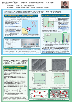
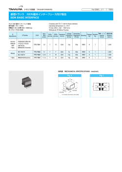
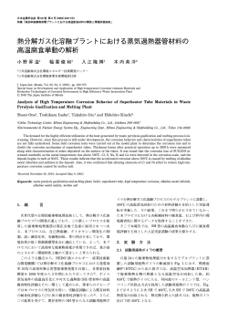
Everything You Always Wanted to Know about Copula
Modeling but Were Afraid to Ask
Christian Genest1 and Anne-Catherine Favre2
Abstract: This paper presents an introduction to inference for copula models, based on rank methods. By working out in detail a small,
fictitious numerical example, the writers exhibit the various steps involved in investigating the dependence between two random variables
and in modeling it using copulas. Simple graphical tools and numerical techniques are presented for selecting an appropriate model,
estimating its parameters, and checking its goodness-of-fit. A larger, realistic application of the methodology to hydrological data is then
presented.
DOI: 10.1061/共ASCE兲1084-0699共2007兲12:4共347兲
CE Database subject headings: Frequency analysis; Distribution functions; Risk management; Statistical models.
F 苸 共F␦兲,
Introduction
Hydrological phenomena are often multidimensional and hence
require the joint modeling of several random variables. Traditionally, the pairwise dependence between variables such as depth,
volume, and duration of flows has been described using classical
families of bivariate distributions. Perhaps the most common
models occurring in this context are the bivariate normal, lognormal, gamma, and extreme-value distributions. The main limitation of this approach is that the individual behavior of the two
variables 共or transformations thereof兲 must then be characterized
by the same parametric family of univariate distributions.
Copula models, which avoid this restriction, are just beginning to make their way into the hydrological literature; see, e.g.,
De Michele and Salvadori 共2002兲, Favre et al. 共2004兲, Salvadori
and De Michele 共2004兲, and De Michele et al. 共2005兲. Restricting
attention to the bivariate case for the sake of simplicity, the
copula approach to dependence modeling is rooted in a representation theorem due to Sklar 共1959兲. The latter states that the joint
cumulative distribution function 共c.d.f.兲 H共x , y兲 of any pair 共X , Y兲
of continuous random variables may be written in the form
H共x,y兲 = C兵F共x兲,G共y兲其,
x,y 苸 R
共1兲
where F共x兲 and G共y兲⫽marginal distributions; and C:关0 , 1兴2
→ 关0 , 1兴⫽copula.
While Sklar 共1959兲 showed that C, F, and G are uniquely
determined when H is known, a valid model for 共X , Y兲 arises from
Eq. 共1兲 whenever the three “ingredients” are chosen from given
parametric families of distributions, viz.
1
Professor, Dépt. de mathématiques et de statistique, Univ. Laval,
Québec QC, Canada G1K 7P4.
2
Professor, Chaire en Hydrologie Statistique, INRS, Eau, Terre et
Environnement, Québec QC, Canada G1K 9A9.
Note. Discussion open until December 1, 2007. Separate discussions
must be submitted for individual papers. To extend the closing date by
one month, a written request must be filed with the ASCE Managing
Editor. The manuscript for this paper was submitted for review and possible publication on August 29, 2006; approved on August 29, 2006. This
paper is part of the Journal of Hydrologic Engineering, Vol. 12, No. 4,
July 1, 2007. ©ASCE, ISSN 1084-0699/2007/4-347–368/$25.00.
G 苸 共G␩兲,
C 苸 共C␪兲
Thus, for example, F might be normal with 共bivariate兲 parameter
␦ = 共␮ , ␴2兲; G might be gamma with parameter ␩ = 共␣ , ␭兲; and C
might be taken from the Farlie–Gumbel–Morgenstern family of
copulas, defined for each ␪ 苸 关−1 , 1兴 by
C␪共u, v兲 = uv + ␪uv共1 − u兲共1 − v兲,
u, v 苸 关0,1兴
共2兲
The main advantage provided to the hydrologist by this approach
is that the selection of an appropriate model for the dependence
between X and Y, represented by the copula, can then proceed
independently from the choice of the marginal distributions.
For an introduction to the theory of copulas and a large selection of related models, the reader may refer, e.g., to the monographs by Joe 共1997兲 and Nelsen 共1999兲, or to reviews such as
Frees and Valdez 共1998兲 and Cherubini et al. 共2004兲, in which
actuarial and financial applications are considered. While the theoretical properties of these objects are now fairly well understood,
inference for copula models is, to an extent, still under development. The literature on the subject is yet to be collated, and most
of it is not written with the end user in mind, making it difficult to
decipher except for the most mathematically inclined.
The aim of this paper is to present, in the simplest terms possible, the successive steps required to build a copula model for
hydrological purposes. To this end, a fictitious data set of 共very兲
small size will be used to illustrate the diagnostic and inferential
tools currently available. Although intuition will be given for the
various techniques to be presented, emphasis will be put on their
implementation, rather than on their theoretical foundation.
Therefore, computations will be presented in more detail than
usual, at the expense of exhaustive mathematical exposition, for
which the reader will only be given appropriate references.
The pedagogical data set to be used throughout the paper is
introduced in the “Dependence and Ranks” section, where it will
be explained why statistical inference concerning dependence
structures should always be based on ranks. This will lead, in the
“Measuring Dependence” section, to the description of classical
nonparametric measures of dependence and tests of independence. Exploratory tools for uncovering dependence and measuring it will be reviewed in the “Additional Graphical Tools for
Detecting Dependence” section. Point and interval estimation for
JOURNAL OF HYDROLOGIC ENGINEERING © ASCE / JULY/AUGUST 2007 / 347
Table 1. Learning Data Set
i
1
2
3
4
5
6
Xi
Yi
−2.224
0.431
−1.538
1.035
−0.807
0.586
0.024
1.465
0.052
1.115
1.324
−0.847
苸 关0 , 1兴. At the other extreme, it can also be shown that in order
for Y to be a deterministic function of X, C must be either one of
the two copulas
W共u, v兲 = max共0,u + v − 1兲
or M共u, v兲 = min共u, v兲
which are usually referred to as the Fréchet–Hoeffding bounds
in the statistical literature; see, e.g., Fréchet 共1951兲 or Nelsen
共1999, p. 9兲. When C = W, Y is a decreasing function of X, while
Y is monotone increasing in X when C = M. More generally,
any copula C represents a model of dependence that lies somewhere between these two extremes, a fact that translates into the
inequalities
W共u, v兲 艋 C共u, v兲 艋 M共u, v兲,
u, v 苸 关0,1兴
To get a feeling for the dependence between X and Y, it is traditional to look at the scatter plot of the pairs 共X1 , Y 1兲 , . . . , 共Xn , Y n兲.
Such a representation is given in Fig. 1共a兲 for the following fictitious random sample of size n = 6 from the bivariate standard
normal distribution with zero correlation. This example will be
used for illustration purposes throughout the paper.
Learning Data Set
Fig. 1. 共a兲 Conventional scatter plot of the pairs 共Xi , Y i兲; 共b兲
corresponding scatter plot of the pairs 共Zi , Ti兲 = 共eXi , e3Y i兲
dependence parameters from copula models will then be presented in the “Estimation” section. Recent goodness-of-fit techniques will be illustrated in the “Goodness-of-Fit Tests” section.
The “Application” section will discuss in detail a concrete hydrological implementation of this methodology. This will lead to the
consideration of additional tools for the treatment of extremevalue dependence structures in the “Graphical Diagnostics for
Bivariate Extreme-Value Copulas” section. Final remarks will
then be made in the “Conclusion” section.
Dependence and Ranks
Suppose that a random sample 共X1 , Y 1兲 , . . . , 共Xn , Y n兲 is given from
some pair 共X , Y兲 of continuous variables, and that it is desired to
identify the bivariate distribution H共x , y兲 that characterizes their
joint behavior. In view of Sklar’s representation theorem, there
exists a unique copula C for which identity, Eq. 共1兲, holds. Therefore, just as F共x兲 and G共y兲 give an exhaustive description of X
and Y taken separately, the joint dependence between these variables is fully and uniquely characterized by C.
It is easy to see, for example, that X and Y are stochastically
independent if and only if C = ⌸, where ⌸共u , v兲 = uv for all u , v
Table 1 shows six independent pairs of mutually independent observations Xi, Y i generated from the standard N共0 , 1兲 distribution
using the statistical freeware R 共R Development Core Team
2004兲. For simplicity, and without loss of generality, the pairs
were labeled in such a way that X1 ⬍ ¯ ⬍ X6.
While there is nothing fundamentally wrong with looking at
the pattern of the pairs 共Xi , Y i兲 共for example, to look for linear
association兲, it must be realized that this picture does not only
incorporate information about the dependence between X and Y,
but also about their marginal behavior. To drive this point home,
consider the transformed pairs
Zi = exp共Xi兲,
Ti = exp共3Y i兲,
1艋i艋6
whose scatter plot, shown in Fig. 1共b兲, is drastically different
from the original one.
In effect, both pictures are distortions of the dependence between the pairs 共X , Y兲 and 共Z , T兲, which is characterized by the
same copula, C, whatever it may be. More generally, if ␸ and ␺
are two increasing transformations with inverses ␸−1 and ␺−1, the
copula of the pair 共Z , T兲 with Z = ␸共X兲 and T = ␺共Y兲 is the same as
that of 共X , Y兲. Let
H*共z,t兲 = C*兵F*共z兲,G*共t兲其
共3兲
be the Sklar representation of the joint distribution of the pair
共Z , T兲. Since the marginal distributions of Z and T are given by
F*共z兲 = P共Z 艋 z兲 = P兵X 艋 ␸−1共z兲其 = F兵␸−1共z兲其
and
348 / JOURNAL OF HYDROLOGIC ENGINEERING © ASCE / JULY/AUGUST 2007
G*共t兲 = P共T 艋 t兲 = P兵Y 艋 ␺−1共t兲其 = G兵␺−1共t兲其
Table 2. Ranks for the Learning Data Set of Table 1
i
1
2
3
4
5
6
Ri
Si
1
2
2
4
3
3
4
6
5
5
6
1
one has
H*共z,t兲 = P共Z 艋 z,T 艋 t兲 = P兵X 艋 ␸−1共z兲,Y 艋 ␺−1共t兲其
=H兵␸−1共z兲,␺−1共t兲其 = C关F兵␸−1共z兲其,G兵␺−1共t兲其兴
=C兵F*共z兲,G*共t兲其
共4兲
for all choices of z , t 苸 R. It follows at once from the comparison
of Eqs. 共3兲 and 共4兲 that C* = C.
Expressed in different terms, the above development means
that the unique copula associated with a random pair 共X , Y兲 is
invariant by monotone increasing transformations of the marginals. Since the dependence between X and Y is characterized by
this copula, a faithful graphical representation of dependence
should exhibit the same invariance property. Among functions of
the data that meet this requirement, it can be seen easily that the
pairs of ranks
共R1,S1兲, . . . ,共Rn,Sn兲
associated with the sample are the statistics that retain the greatest
amount of information; see, e.g., Oakes 共1982兲. Here, Ri stands
for the rank of Xi among X1 , . . . , Xn, and Si stands for the rank of
Y i among Y 1 , . . . , Y n. These ranks are unambiguously defined, because ties occur with probability zero under the assumption of
continuity for X and Y. Pairs of ranks corresponding to the learning data set are given in Table 2.
Displayed in Fig. 2共a兲 is the scatter plot of the pairs 共Ri , Si兲
corresponding to these 共Xi , Y i兲. Fig. 2共b兲 shows the graph of the
pairs 共R*i , S*i 兲 associated with the 共Zi , Ti兲. The result is obviously
the same. It is the most judicious representation of the copula C
that one could hope for. Upon rescaling of the axes by a factor of
1 / 共n + 1兲, one gets a set of points in the unit square 关0 , 1兴2, which
form the domain of the so-called empirical copula 共Deheuvels
1979兲, formally defined by
n
冉
1
Ri
Si
艋 u,
艋v
1
Cn共u, v兲 =
n i=1 n + 1
n+1
兺
冊
with 1共A兲 denoting the indicator function of set A. For any given
pair 共u , v兲, it may be shown that Cn共u , v兲 is a rank-based estimator of the unknown quantity C共u , v兲 whose large-sample distribution is centered at C共u , v兲 and normal.
Fig. 2. Displayed in 共a兲 is a scatter plot of the pairs 共Ri , Si兲 of ranks
derived from the learning data set 共Xi , Y i兲, 1 艋 i 艋 6. As for 共b兲, it
shows a scatter plot of the pairs 共R*i , S*i 兲 of ranks derived from the
transformed data 共Zi , Ti兲 = 共exp共Xi兲 , exp共3Y i兲兲, 1 艋 i 艋 6. For obvious
reasons, the two graphs are actually identical.
tween the pairs 共Ri , Si兲 of ranks, or equivalently between the
points 共Ri / 共n + 1兲 , Si / 共n + 1兲兲 forming the support of Cn. This leads
directly to Spearman’s rho, viz.
Measuring Dependence
n
It was argued above that the empirical copula Cn is the best
sample-based representation of the copula C, which is itself a
characterization of the dependence in a pair 共X , Y兲. It would make
sense, therefore, to measure dependence, both empirically and
theoretically, using Cn and C, respectively. It will now be explained how this leads to two well-known nonparametric measures of dependence, namely Spearman’s rho and Kendall’s tau.
␳n =
共Ri − ¯R兲共Si − ¯S兲
兺
i=1
冑兺
n
苸 关− 1,1兴
n
共Ri − ¯R兲2
i=1
共Si − ¯S兲2
兺
i=1
where
n
n
¯R = 1 R = n + 1 = 1 S = ¯S
i
i
2
n i=1
n i=1
兺
Spearman’s Rho
Mimicking the familiar approach of Pearson to the measurement
of dependence, a natural idea is to compute the correlation be-
兺
This coefficient, which may be expressed more conveniently in
the form
JOURNAL OF HYDROLOGIC ENGINEERING © ASCE / JULY/AUGUST 2007 / 349
n
␳n =
12
n+1
R iS i − 3
n共n + 1兲共n − 1兲 i=1
n−1
兺
shares with Pearson’s classical correlation coefficient, rn, the
property that its expectation vanishes when the variables are independent. However, ␳n is theoretically far superior to rn, in that
1. E共␳n兲 = ± 1 occurs if and only if X and Y are functionally
dependent, i.e., whenever their underlying copula is one of
the two Fréchet–Hoeffding bounds, M or W;
2. In contrast, E共rn兲 = ± 1 if and only if X and Y are linear
functions of one another, which is much more restrictive; and
3. ␳n estimates a population parameter that is always well defined, whereas there are heavy-tailed distributions 共such as
the Cauchy, for example兲 for which a theoretical value of
Pearson’s correlation does not exist.
For additional discussion on these points, see, e.g., Embrechts
et al. 共2002兲.
As it turns out, ␳n is an asymptotically unbiased estimator of
␳ = 12
冕
关0,1兴2
uvdC共u, v兲 − 3 = 12
冕
关0,1兴2
C共u, v兲dvdu − 3
where the second equality is an identity originally proven by
Hoeffding 共1940兲 and extended by Quesada-Molina 共1992兲. To
show this, one may use the fact that
冕
n
n−1
12
Ri Si
12
−3=
␳n
uvdCn共u, v兲 − 3 =
n i=1 n + 1 n + 1
n+1
关0,1兴2
兺
and that Cn → C as n → ⬁. For more precise conditions under
which this result holds, see, e.g., Hoeffding 共1948兲.
Note in passing that under the null hypothesis H0 : C = ⌸
of independence between X and Y, the distribution of ␳n is
close to normal with zero mean and variance 1 / 共n − 1兲, so that
one may reject H0 at approximate level ␣ = 5%, for instance, if
冑n − 1 兩 ␳n 兩 ⬎ z␣/2 = 1.96.
Example
For the observations from the learning data set, a simple calculation yields ␳n = 1 / 35= 0.028, while rn = −0.397. Here, there is no
reason to reject the null hypothesis of independence. For, if Z is a
standard normal random variable, the P-value of the test based on
␳n is 2Pr共Z ⬎ 冑5 / 35兲 = 94.9%.
Given a family 共C␪兲 of copulas indexed by a real parameter,
the theoretical value of ␳ is, typically, a monotone increasing
function of ␪. A sufficient condition for this is that the copulas be
ordered by positive quadrant dependence 共PQD兲, which means
that the implication ␪ ⬍ ␪⬘ ⇒ C␪共u , v兲 艋 C␪⬘共u , v兲 is true for all
u , v 苸 关0 , 1兴. The original definition of PQD as a concept of
dependence goes back to Lehmann 共1966兲; the same ordering,
rediscovered by Dhaene and Goovaerts 共1996兲 in an actuarial
context, is often referred to as the correlation or concordance
ordering in that field.
In the Farlie–Gumbel–Morgenstern model, for example, one
has
冕
关0,1兴2
where
冕冕
1
uvdC␪共u, v兲 =
0
1
0
uvc␪共u, v兲dvdu
Fig. 3. Spearman’s rho 共a兲 and Kendall’s tau 共b兲 as a function of
Pearson’s correlation in the bivariate normal model
⳵2
C␪共u, v兲 = 1 + ␪共1 − 2u兲共1 − 2v兲
⳵u⳵v
c␪共u, v兲 =
since C␪ is absolutely continuous in this case. A simple calculation then yields
冕冕
1
0
1
0
uvc␪共u, v兲dvdu =
1 ␪
+
4 36
and, hence, ␳ = ␪ / 3, as initially shown by Schucany et al. 共1978兲.
As a second example, if 共X , Y兲 follows a bivariate normal distribution with correlation r, a somewhat intricate calculation to be
found, e.g., in Kruskal 共1958兲, shows that
冕冕
⬁
␳ = 12
−⬁
⬁
−⬁
F共x兲G共y兲dH共x,y兲 − 3 =
冉冊
6
r
arcsin
␲
2
For those people accustomed to thinking in terms of r, the above
formula may suggest that a serious effort would be required to
think of correlation in terms of Spearman’s rho in the traditional
bivariate normal model. As shown in Fig. 3共a兲, however, the difference between ␳ and r is minimal in this context.
350 / JOURNAL OF HYDROLOGIC ENGINEERING © ASCE / JULY/AUGUST 2007
¯ =
W
冕
关0,1兴2
Cn共u, v兲dCn共u, v兲
Using Eq. 共6兲 and the fact that under suitable regularity conditions, Cn → C as n → ⬁, one can conclude 关with Hoeffding 共1948兲兴
that ␶n is an asymptotically unbiased estimator of the population
version of Kendall’s tau, given by
␶=4
Fig. 4. Two pairs of concordant 共a兲 and discordant 共b兲 observations
冑
A second, well-known measure of dependence based on ranks is
Kendall’s tau, whose empirical version is given by
冉冊
共5兲
where Pn and Qn = number of concordant and discordant pairs,
respectively. Here, two pairs 共Xi , Y i兲, 共X j , Y j兲 are said to be
concordant when 共Xi − X j兲共Y i − Y j兲 ⬎ 0, and discordant when
共Xi − X j兲共Y i − Y j兲 ⬍ 0. One need not worry about ties, since the borderline case 共Xi − X j兲共Y i − Y j兲 = 0 occurs with probability zero
under the assumption that X and Y are continuous. The characteristic patterns of concordant and discordant pairs are displayed in
Fig. 4.
It is obvious that ␶n is a function of the ranks of the observations only, since 共Xi − X j兲共Y i − Y j兲 ⬎ 0 if and only if 共Ri − R j兲
⫻共Si − S j兲 ⬎ 0. Accordingly, ␶n is also a function of Cn. To make
the connection, introduce
Iij =
再
1
0
if X j ⬍ Xi,Y j ⬍ Y i
otherwise
冎
for arbitrary i ⫽ j, and let Iii = 1 for all i 苸 兵1 , . . . , n其. Observe that
n
n
1
Pn =
2 i=1
n
共Iij + I ji兲 = 兺 兺 Iij = − n + 兺 兺 Iij
兺兺
j⫽i
i=1 j⫽i
i=1 j=1
n
1
1
Iij = # 兵j:X j 艋 Xi,Y j 艋 Y i其
n j=1
n
兺
¯ = 共W + ¯ + W 兲 / n, then P = −n + n2W
¯ and
so that if W
1
n
n
␶n = 4
n ¯ n+3
W−
n−1
n−1
共6兲
The connection with Cn then comes from the fact that by
definition
Wi = Cn
hence
冉
Ri
Si
,
n+1 n+1
冊
9n共n − 1兲
兩␶n兩 ⬎ 1.96
2共2n + 5兲
冕
冕冕
1
关0,1兴2
C␪共u, v兲dC␪共u, v兲 =
0
1
C␪共u, v兲c␪共u, v兲dvdu
0
which reduces to ␪ / 18+ 1 / 4, hence ␶ = 2␪ / 9, as per Schucany
et al. 共1978兲.
For the bivariate normal model with correlation r, Kruskal
共1958兲 has shown that
冕冕
⬁
␶=4
⬁
H共x,y兲dH共x,y兲 − 1 =
−⬁
2
arcsin共r兲
␲
As shown in Fig. 3共b兲, ␶ is also nearly a linear function of r in this
special case.
since Iij + I ji = 1 if and only if the pairs 共Xi , Y i兲 and 共X j , Y j兲 are
concordant.
Now write
Wi =
C共u, v兲dC共u, v兲 − 1
Example (Continued)
For the observations from the learning data set, a simple calculation yields ␶n = 1 / 15= 0.067. Here, there is no reason to reject
the null hypothesis of independence. For, if Z is a standard normal random variable, the P-value of the test based on ␶n is
2Pr共Z ⬎ 0.188兲 = 85.1%.
As for Spearman’s rho, the theoretical value of Kendall’s tau is
a monotone increasing function of the real parameter ␪ whenever
a family 共C␪兲 of copulas is ordered by positive quadrant dependence. In the Farlie–Gumbel–Morgenstern model, for example,
one has
−⬁
n
关0,1兴2
An alternative test of independence can be based on ␶n, since
under H0, this statistic is close to normal with zero mean and
variance 2共2n + 5兲 / 兵9n共n − 1兲其. Thus, H0 would be rejected at approximate level ␣ = 5% if
Kendall’s Tau
Pn − Qn
4
␶n =
Pn − 1
=
n共n − 1兲
n
2
冕
Other Measures and Tests of Dependence
Although Spearman’s rho and Kendall’s tau are the two most
common statistics with which dependence is measured and tested,
many alternative rank-based procedures have been proposed in
the statistical literature. Most of them are based on expressions of
the form
冕
J共u, v兲dCn共u, v兲
where J is some 共suitably regular兲 score function. Thus, while
J共u , v兲 = uv is the basis of Spearman’s statistic, as seen earlier, the
choice J共u , v兲 = ⌽−1共u兲⌽−1共v兲, e.g., yields the van der Waerden
statistic. Genest and Verret 共2005兲, who review this literature,
explain how each J should be chosen so as to yield the most
powerful testing procedure against a specific class of copula alternatives.
JOURNAL OF HYDROLOGIC ENGINEERING © ASCE / JULY/AUGUST 2007 / 351
In the absence of privileged information about the suspected
departure from independence, however, omnibus procedures such
as those based on ␳n and ␶n usually perform well. See Deheuvels
共1981兲 or Genest and Rémillard 共2004兲 for other general tests
based on the empirical copula process Cn = 冑n共Cn − C兲.
Additional Graphical Tools for Detecting
Dependence
Besides the scatter plot of ranks, two graphical tools for detecting
dependence have recently been proposed in the literature, namely,
chi-plots and K-plots. These will be briefly described in turn.
Chi-Plots
Chi-plots were originally proposed by Fisher and Switzer 共1985兲
and more fully illustrated in Fisher and Switzer 共2001兲. Their
construction is inspired from control charts and based on the chisquare statistic for independence in a two-way table. Specifically,
introduce
Hi =
1
nWi − 1
# 兵j ⫽ i:X j 艋 Xi,Y j 艋 Y i其 =
n−1
n−1
Fi =
1
# 兵j ⫽ i:X j 艋 Xi其
n−1
Gi =
1
# 兵j ⫽ i:Y j 艋 Y i其
n−1
and
Noting that these quantities depend exclusively on the ranks of
the observations, Fisher and Switzer propose to plot the pairs
共␭i , ␹i兲, where
␹i =
H i − F iG i
冑Fi共1 − Fi兲Gi共1 − Gi兲
Fig. 5. Chi-plot for the learning data set
tional chi-square test statistic for independence in the two-way
table generated by counting points in the four regions delineated
by the lines x = Xi and y = Y i.
Since one would expect Hi ⬇ Fi ⫻ Gi for all i under independence, values of ␹i that fall too far from zero are indicative of
departures from that hypothesis. To help identify such departures,
Fisher and Switzer 共1985, 2001兲 suggest that “control limits” be
drawn at ±c p / 冑n, where c p is selected so that approximately
100p% of the pairs 共␭i , ␹i兲 lie between the lines. Through simulations, they found that the c p values 1.54, 1.78, and 2.18 correspond to p = 0.9, 0.95, and 0.99, respectively.
K-Plots
Another rank-based graphical tool for visualizing dependence was
recently proposed by Genest and Boies 共2003兲. It is inspired by
the familiar notion of QQ-plot. Specifically, their technique consists in plotting the pairs 共Wi:n , H共i兲兲 for i 苸 兵1 , . . . , n其, where
H共1兲 ⬍ ¯ ⬍ H共n兲
and
˜G
˜
˜2 ˜ 2
␭i = 4 sign 共F
i i兲 max 共Fi ,Gi 兲
˜ = G − 1 / 2 for i 苸 兵1 , . . . , n其. To avoid
where ˜Fi = Fi − 1 / 2, G
i
i
outliers, they recommend that what should be plotted are only the
pairs for which
兩␭i兩 艋 4
冉
1
1
−
n−1 2
冊
are the order statistics associated with the quantities H1 , . . . , Hn
introduced in the “Chi-Plots” subsection. As for Wi:n, it is the
expected value of the ith statistic from a random sample of size n
from the random variable W = C共U , V兲 = H共X , Y兲 under the null
hypothesis of independence between U and V 共or between X and
Y, which is the same兲. The latter is given by
2
Fig. 5 shows the resulting graph for the learning data set of
Tables 1 and 2. The coordinates of the points and the intermediate
calculations that lead to them are summarized in Table 3. Note
that, in general, between two and four points may be lost due to
division by zero; such is the case here for three points. Given that
the original data set consisted of six observations only, this leaves
only 6 − 3 = 3 points on the graph, which is obviously not particularly revealing. However, the real-life applications considered in
the “Application” section and by Fisher and Switzer 共1985, 2001兲
provide more convincing evidence of the usefulness of this tool.
Fisher and Switzer 共1985, 2001兲 argue that ␭i, ␹i 苸 关−1 , 1兴.
While ␭i = measure of distance between the pair 共Xi , Y i兲 and the
center of the scatter plot, 冑n␹i = 共signed兲 square root of the tradi-
Wi:n = n
冉 冊冕
n−1
i−1
1
wk0共w兲兵K0共w兲其i−1兵1 − K0共w兲其n−idw
0
where
Table 3. Computations Required for Drawing the Chi-Plot Associated
with the Learning Data Set of Table 1
i
1
2
3
4
5
6
5Hi
5Fi
5Gi
␹i
␭i
0
0
1
—
1
1
1
3
0.408
−0.36
1
2
2
0.167
0.04
3
3
5
—
1
3
4
4
−0.25
0.36
0
5
0
—
−1
352 / JOURNAL OF HYDROLOGIC ENGINEERING © ASCE / JULY/AUGUST 2007
Table 4. Coordinates of Points Displayed on the K-Plot Associated with
the Learning Data Set of Table 1
i
Wi:6
H共i兲
1
2
3
4
5
6
0.038
0.0
0.092
0.2
0.163
0.2
0.256
0.6
0.381
0.6
0.569
0.0
thus rely only on the ranks of the observations, which are the best
summary of the joint behavior of the random pairs.
Estimate Based on Kendall’s Tau
Fig. 6. K-plot for the learning data set. Superimposed on the graph
are a straight line corresponding to the case of independence and a
smooth curve K0共w兲 associated with perfect positive dependence.
冕 冉
1
K0共w兲 = P共UV 艋 w兲 =
=
冕
w
0
1dv +
冕
P U艋
0
1
w
To fix ideas, suppose that the underlying dependence structure
of a random pair 共X , Y兲 is appropriately modeled by the Farlie–
Gumbel–Morgenstern family 共C␪兲 defined in Eq. 共2兲. In this case,
␪ is real and as seen in the “Kendall’s Tau” subsection there exists
an immediate relation in this model between the parameter ␪ and
the population value ␶ of Kendall’s tau, namely
2
␶= ␪
9
冊
Given a sample value ␶n of ␶ computed from Eq. 共5兲 or 共6兲, a
simple and intuitive approach to estimating ␪ would then consist
of taking
w
dv
v
w
dv = w − w log共w兲
v
˜␪ = 9 ␶
n
n
2
and k0 = corresponding density.
The values of W1:6 , . . . , W6:6 required to produce Fig. 6 can be
readily computed using any symbolic calculator, such as Maple.
They are given in Table 4. The interpretation of K-plots is similar
to that of QQ-plots: just as curvature is problematic, e.g., in a
normal QQ-plot, any deviation from the main diagonal is a sign
of dependence in K-plots. Positive or negative dependence may
be suspected in the data, depending whether the curve is located
above or below the line y = x. Roughly speaking, “the further the
distance, the greater the dependence.” In this construction, perfect
negative dependence 共i.e., C = W兲 would translate into a string of
data points aligned on the x-axis. As for perfect positive dependence 共i.e., C = M兲, it would materialize into data aligned on the
curve K0共w兲 shown on the graph.
As for the chi-plot, the linearity 共or lack thereof兲 in the K-plot
displayed in Fig. 6 is hard to detect, given the extremely small
size of the learning data set. However, see the “Application” section and Genest and Boies 共2003兲 for more compelling illustrartions of K-plots.
Since ␶n is rank-based, this estimation strategy may be construed
as a nonparametric adaptation of the celebrated method of
moments.
More generally, if ␪ = g共␶兲 for some smooth function g, then
˜␪ = g共␶ 兲 may be referred to as the Kendall-based estimator of ␪.
n
n
A small adaptation of Proposition 3.1 of Genest and Rivest 共1993兲
implies that
Estimation
Therefore, an application of Slutsky’s theorem, also known as the
“Delta method,” implies that as n → ⬁
Now suppose that a parametric family 共C␪兲 of copulas is being
considered as a model for the dependence between two random
variables X and Y. Given a random sample 共X1 , Y 1兲 , . . . , 共Xn , Y n兲
from 共X , Y兲, how should ␪ be estimated? This section reviews
different nonparametric strategies for tackling this problem, depending on whether ␪ is real or multidimensional.
Only rank-based estimators are considered in the sequel. This
methodological choice is justified by the fact, highlighted earlier,
that the dependence structure captured by a copula has nothing to
do with the individual behavior of the variables. A fortiori, any
inference about the parameter indexing a family of copulas should
冑n ␶n − ␶ ⬇ N共0,1兲
4S
where
n
S2 =
1
˜ − 2W
¯ 兲2
共Wi + W
i
n i=1
兺
and
n
˜ = 1 I = 1 # 兵j:X 艋 X ,Y 艋 Y 其
W
i
ji
i
j i
j
n j=1
n
兺
冋
˜␪ ⬇ N ␪, 1 兵4Sg⬘共␶ 兲其2
n
n
n
册
Accordingly, an approximate 100⫻ 共1 − ␣兲% confidence interval
for ␪ is given by
˜␪ ± z 1 4S兩g⬘共␶ 兲兩
n
␣/2
n
冑n
For an alternative consistent estimator of the asymptotic variance
of ␶n, see for instance, Samara and Randles 共1988兲.
JOURNAL OF HYDROLOGIC ENGINEERING © ASCE / JULY/AUGUST 2007 / 353
Table 5. Intermediate Values Required for the Computation of the
Standard Error Associated with Kendall’s Tau
i
1
2
3
4
5
6
6Wi
˜
6W
1
5
2
3
2
3
4
1
4
1
1
1
i
Table 6. Three Common Families of Archimedean Copulas, Their
Generator, Their Parameter Space, and an Expression for the Population
Value of Kendall’s Tau
Family
Generator
Parameter
Kendall’s tau
Clayton
共t − 1兲 / ␪
␪ 艌 −1
␪ / 共␪ + 2兲
␪苸R
1 − 4 / ␪ + 4D1共␪兲 / ␪
␪艌1
1−1/␪
−␪
Frank
Example (Continued)
For the learning data set of Table 1, it was seen earlier that
␶n = 1 / 15, hence ˜␪n = 0.3. Using the intermediate quantities summarized in Table 5, one finds S2 = 0.043, hence an approximate
95% confidence interval for this estimation is 关−1 , 1兴, since
g⬘共␶兲 ⬅ 9 / 2, and hence, 1.96⫻ 4S兩g⬘共␶n兲兩 / 冑n = 2.99. While the
size of the standard error may appear exceedingly conservative,
this result is not surprising, considering that the sample size is
n = 6.
The popularity of ˜␪n as an estimator of the dependence parameter stems in part from the fact that closed-form expressions for
the population value of Kendall’s tau are available for many
common parametric copula models. Such is the case, in particular,
for several Archimedean families of copulas, e.g., those of Ali
et al. 共1978兲, Clayton 共1978兲, Frank 共1979兲, Gumbel–Hougaard
共Gumbel 1960兲, etc. Specifically, a copula C is said to be
Archimedean if there exists a convex, decreasing function
␸ : 共0 , 1兴 → 关0 , ⬁兲 such that ␸共1兲 = 0 and
C共u, v兲 = ␸−1兵␸共u兲 + ␸共v兲其
is valid for all u , v 苸 共0 , 1兲. As shown by Genest and MacKay
共1986兲
␶=1+4
冕
1
0
␸共t兲
dt
␸⬘共t兲
Note: Here,
共
冋
1
␪˘ n ⬇ N ␪, 兵␴nh⬘共␳n兲其2
n
␴2
n
where the asymptotic variance ␴2 depends on the underlying
copula C in a way that has been described in detail by Borkowf
共2002兲. Arguing along the same lines as in the “Estimate Based on
册
where ␴2n = suitable estimator of ␴2. An approximate 100⫻ 共1
− ␣兲% confidence interval for ␪ is then given by
1
␪˘ n ± z␣/2 ␴n兩h⬘共␳n兲兩
冑n
Substituting Cn for C in the expressions reported by Borkowf
共2002兲, a very natural, consistent estimate for ␴2 is given by
␴2n = 144共− 9A2n + Bn + 2Cn + 2Dn + 2En兲
where
n
1
Ri Si
n i=1 n + 1 n + 1
兺
An =
n
冉 冊冉 冊
1
Ri
Bn =
n i=1 n + 1
兺
n
Cn =
1
n3 i=1
n
n
R
2
Si
n+1
2
1
S
i
i
1共Rk 艋 Ri,Sk 艋 S j兲 + − An
兺
兺兺
4
n
+
1
n
+
1
j=1 k=1
n
n
n
n
Dn =
1
n2 i=1
En =
1
n2 i=1
S
S
冉
Ri
Rj
,
n+1 n+1
R
R
冉
Si
Sj
,
n+1 n+1
i
j
max
兺兺
j=1 n + 1 n + 1
冊
and
␪˘ n = h共␳n兲
冉 冊
is the first Debye function.
Kendall’s Tau” subsection, it can then be seen that under suitable
regularity conditions on h
Estimate Based on Spearman’s Rho
where ␪ = h共␳兲 represents the relationship between the parameter
and the population value of Spearman’s rho. In the context of the
Farlie–Gumbel–Morgenstern family of copulas, for example, it
was seen earlier that ␳ = ␪ / 3, so that ␪˘ n = 3␳n would be an alternative nonparametric estimator to ˜␪n = 9␶n / 2.
Now it follows from standard convergence results about empirical processes to be found, e.g., in Chapter 5 of Gaenssler and
Stute 共1987兲, that
兲
D1共␪兲 = 兰␪0共x / ␪兲 / 共ex − 1兲dx
共7兲
When the dependence parameter ␪ is real, an alternative rankbased estimator that remains in the spirit of the method of moments consists of taking
e−␪t − 1
e−␪ − 1
兩log共t兲兩␪
Gumbel–Hougaard
Table 6 gives the generator ␸ and an expression for ␶ for the
three most common Archimedean models. Algebraically closed
formulas are available for various other dependence models,
e.g., extreme-value or Archimax copulas. See, for example,
Ghoudi et al. 共1998兲 or Capéraà et al. 共2000兲.
␳n ⬇ N ␳,
−log
i
j
max
兺兺
n
+
1
n
+
1
j=1
冊
Example (Continued)
For the learning data set of Table 1, it was seen earlier that
␳n = 1 / 35, hence ␪˘ n = 3 / 35⬇ 0.086. Burdensome but simple
calculations yield ␴n = 7.77, hence an approximate 95% confidence interval for this estimation is 关−1 , 1兴, since h⬘共␶兲 ⬅ 3,
and hence, 1.96⫻ ␴n兩h⬘共␳n兲兩 / 冑n = 18.66. Here again, the size of
the standard error is quite large, as might be expected given
that n = 6.
Maximum Pseudolikelihood Estimator
In classical statistics, maximum likelihood estimation is a wellknown alternative to the method of moments that is usually more
354 / JOURNAL OF HYDROLOGIC ENGINEERING © ASCE / JULY/AUGUST 2007
efficient, particularly when ␪ is multidimensional. In the present
context, an adaptation of this approach to estimation is required if
inference concerning dependence parameters is to be based exclusively on ranks. Such an adaptation was described in broad terms
by Oakes 共1994兲 and was later formalized and studied by Genest
et al. 共1995兲 and by Shih and Louis 共1995兲.
The method of maximum pseudolikelihood, which requires
that C␪ be absolutely continuous with density c␪, simply involves
maximizing a rank-based, log-likelihood of the form
n
ᐉ共␪兲 =
log
兺
i=1
再冉
c␪
Si
Ri
,
n+1 n+1
冊冎
共8兲
The latter is exactly the expression one gets when the unknown
marginal distributions F and G in the classical log-likelihood
n
ᐉ共␪兲 =
log关c␪兵F共Xi兲,G共Y i兲其兴
兺
i=1
are replaced by rescaled versions of their empirical counterparts,
i.e.
n
␴ˆ 2n =
n
1
¯ 兲2
共Ni − N
␤ˆ 2n =
n i=1
兺
are sample variances computed from two sets of pseudo¯ = 共M + ¯ + M 兲 / n
observations
with
means
M
and
1
n
¯ = 共N + ¯ + N 兲 / n, respectively.
N
1
n
To compute the pseudo-observations M i and Ni, one should
proceed as follows:
• Step 1: Relabel the original data 共X1 , Y 1兲 , . . . , 共Xn , Y n兲 in such
a way that X1 ⬍ ¯ ⬍ Xn; as a consequence one then has
R1 = 1 , . . . , Rn = n.
• Step 2: Write L共␪ , u , v兲 = log c␪共u , v兲 and compute L␪, Lu, and
Lv, which are the derivatives of L with respect to ␪, u, and v,
respectively.
• Step 3: For i 苸 兵1 , . . . , n其, set
冉
Ni = L␪ ␪ˆ n,
兺
M i = Ni −
n
1
1共Y i 艋 y兲
Gn共y兲 =
n + 1 i=1
兺
That this substitution yields formula 共8兲 is immediate, once it
is realized that Fn共Xi兲 = Ri / 共n + 1兲 and Gn共Y i兲 = Si / 共n + 1兲 for all
i 苸 兵1 , . . . , n其.
This method may seem superficially less attractive than the
inversion of Kendall’s tau or Spearman’s rho, both because it
involves numerical work and requires the existence of a density
c␪. At the same time, however, it is much more generally applicable than the other methods, since it does not require the dependence parameter to be real. The procedure for estimating a
multivariate ␪ and computing associated approximate confidence
region is described by Genest et al. 共1995兲. For simplicity, it is
only presented here in the case where ␪ is real; however, see the
“Application” section for the bivariate case.
Letting c˙␪共u , v兲 = ⳵c␪共u , v兲 / ⳵␪, Genest et al. 共1995兲 show under
mild regularity conditions that the root ␪ˆ n of the equation
⳵
ᐉ˙ 共␪兲 = ᐉ共␪兲 =
⳵␪
兺
i=1
c␪
冉
冉
冊
冊
−
1
n
n
L␪
兺
j=i
冉
冉
␪ˆ n,
冊冉
冊冉
Sj
Sj
j
j
,
,
Lu ␪ˆ n,
n+1 n+1
n+1 n+1
兺
c␪共u, v兲 = 1 + ␪共1 − 2u兲共1 − 2v兲
and
共1 − 2u兲共1 − 2v兲
c˙␪共u, v兲
=
c␪共u, v兲 1 + ␪共1 − 2u兲共1 − 2v兲
Accordingly, the log-pseudolikelihood associated with this model
is given by
n
log
兺
i=1
n
ᐉ˙ 共␪兲 =
冉 冊
␯2
␪ˆ n ⬇ N ␪,
n
兺
i=1
n
where ␯2 depends exclusively on the true underlying copula C␪ as
per Proposition 2.1 of Genest et al. 共1995兲. As mentioned by these
authors, a consistent estimate of ␯2 is given by
冊
冊
Example (Continued)
Suppose that a Farlie–Gumbel–Morgenstern copula model is
being considered for the learning data set of Table 1. In this case
再 冉
1+␪ 1−
2Ri
n+1
冊冉
1−
and the corresponding pseudoscore function is
is unique. Furthermore
where
冊
1
Sj
Sj
j
j
,
,
L␪ ␪ˆ n,
Lv ␪ˆ n,
n S j艌Si
n+1 n+1
n+1 n+1
ᐉ共␪兲 =
Ri
Si
,
n+1 n+1
=0
Ri
Si
,
n+1 n+1
␯ˆ 2n = ␴ˆ 2n/␤ˆ 2n
Si
i
,
n+1 n+1
• Step 4: For i 苸 兵1 , . . . , n其, let also
and
c˙␪
兺
and
n
1
1共Xi 艋 x兲
Fn共x兲 =
n + 1 i=1
n
1
¯ 兲2
共M i − M
n i=1
=
冉
冊冉
冊冉
2Si
n+1
冊
Ri
Si
1−2
n+1
n+1
Ri
Si
1+␪ 1−2
1−2
n+1
n+1
1−2
冉
冊冎
冊
共n + 1 − 2R 兲共n + 1 − 2S 兲
i
i
兺
2
共n
+
1兲
+
␪共n
+
1
−
2R
兲共n
+
1
− 2Si兲
i
i=1
These two functions are plotted in Fig. 7 with n = 6 and the values
of Ri and Si given in Table 2.
Upon substitution, one gets ␪ˆ n = 0.0989 as the unique root of
the equation
JOURNAL OF HYDROLOGIC ENGINEERING © ASCE / JULY/AUGUST 2007 / 355
Table 7. Values of the Constants Ni and M i Required to Compute an
Approximate Confidence Interval for the Maximum of Pseudolikelihood
Estimator ␪ˆ
n
i
Ni
Mi
1
2
3
4
5
6
0.297
0.286
−0.0616
−0.0832
0.0204
−0.00147
0.101
0.0824
0.180
0.162
−0.537
−0.534
one gets ␯ˆ 2n = 0.0677/ 0.0707= 0.958 and 1.96⫻ ␯ˆ n / 冑n = 0.783. The
confidence interval for the maximum likelihood estimator is given
by 关−0.684, 0.882兴.
Other Estimation Methods
Fig. 7. Graphs of ᐉ共␪兲 共a兲 and ᐉ˙ 共␪兲 共b兲 for the learning data set of
Table 1 when the assumed model is the Farlie–Gumbel–Morgenstern
family of copulas
ᐉ˙ 共␪兲 =
3
1
5
15
−
+
+
49 + 15␪ 49 − 3␪ 49 + ␪ 49 + 5␪
+
25
9
−
=0
49 + 9␪ 49 − 25␪
In the present case
L␪共␪,u, v兲 =
共1 − 2u兲共1 − 2v兲
1 + ␪共1 − 2u兲共1 − 2v兲
Lu共␪,u, v兲 =
− 2␪共1 − 2v兲
1 + ␪共1 − 2u兲共1 − 2v兲
Lv共␪,u, v兲 =
− 2␪共1 − 2u兲
1 + ␪共1 − 2u兲共1 − 2v兲
Using the intermediate calculations summarized in Table 7,
Although they are the most common, estimators based on the
maximization of the pseudolikelihood and on the inversion of
either Kendall’s tau or Spearman’s rho are not the only rankbased procedures available for selecting appropriate values of dependence parameters in a copula-based model. Tsukahara 共2005兲,
for example, recently investigated the behavior and performance
of two new classes of estimators derived from minimum-distance
criteria and an estimating-equation approach. In his simulations,
however, the maximum pseudolikelihood estimator turned out to
have the smallest mean-squared error. Circumstances under which
the latter approach is asymptotically semiparametrically efficient
were delineated by Klaassen and Wellner 共1997兲 and by Genest
and Werker 共2002兲. See Biau and Wegkamp 共2005兲 for another
rank-based, minimum-distance method for dependence parameter
estimation.
In all fairness, it should be mentioned that the exclusive reliance on ranks for copula parameter estimation advocated here
does not make complete consensus in the statistical community.
In his book, Joe 共1997, Chap. 10兲 recommends a parametric twostep procedure often referred to as the “inference from margins”
or IFM method. As in the pseudolikelihood approach described
above, the estimate of ␪ is obtained through the maximization of
a function of the form
n
ᐉ共␪兲 =
ˆ 共Y 兲其兴
log关c␪兵Fˆ共Xi兲,G
i
兺
i=1
ˆ =G ,
However, while the rank-based method takes Fˆ = Fn and G
n
ˆ = G , where 共F 兲 and
Joe 共1997兲 substitutes Fˆ = F␦n and G
␩n
␦
共G␩兲 = suitable parametric families for the margins, and ␦n
and ␩n = standard maximum likelihood estimates of their parameters, derived from the observed values of X and Y, respectively.
Cherubini et al. 共2004, Section 5.3兲 point out that the IFM method
may be viewed as a special case of the generalized method of
moments with an identity weight matrix. Joe 共2005兲 quantifies the
asymptotic efficiency of the approach in different circumstances.
Although they usually perform well, the estimates of the association parameters derived by the IFM technique clearly depend on
the choice of F and G, and thus always run the risk of being
unduly affected if the models selected for the margins turn out to
be inappropriate 关see e.g., Kim et al. 共2007兲兴.
For completeness, it may be worth mentioning that another
developing body of literature proposes the use of kernel methods
to derive a smooth estimate of a copula or its density, without
assuming any specific parametric form for it. See, e.g., Gijbels
and Mielniczuk 共1990兲 or Fermanian and Scaillet 共2003兲.
356 / JOURNAL OF HYDROLOGIC ENGINEERING © ASCE / JULY/AUGUST 2007
Goodness-of-Fit Tests
In typical modeling exercises, the user has a choice between several different dependence structures for the data at hand. To keep
things simple, suppose that two copulas C␪n and D␰n were fitted
by some arbitrary method. It is then natural to ask which of the
two models provides the best fit to the observations. Both informal and formal ways of tackling this question will be discussed in
turn.
Graphical Diagnostics
When dealing with bivariate data, possibly the most natural way
of checking the adequacy of a copula model would be to compare
a scatter plot of the pairs 共Ri / 共n + 1兲 , Si / 共n + 1兲兲 共i.e., the support
of the empirical copula Cn兲 with an artificial data set of the same
size generated from C␪n. To avoid arbitrariness induced by sampling variability, however, a better strategy consists of generating
a large sample from C␪n, which effectively amounts to portraying
the associated copula density in two dimensions.
Simple simulation algorithms are available for most copula
models; see, e.g., Devroye 共1986, Chap. 11兲, or Whelan 共2004兲
for Archimedean copulas. In the bivariate case, a good strategy
for generating a pair 共U , V兲 from a copula C proceeds as follows:
• Step 1: Generate U from a uniform distribution on the interval
共0, 1兲.
• Step 2: Given U = u, generate V from the conditional
distribution
Qu共v兲 = P共V 艋 v兩U = u兲 =
⳵
C共u, v兲
⳵u
*
*
by setting V = Q−1
u 共U 兲, where U = another observation from
the uniform distribution on the interval 共0, 1兲. When an ex−1 *
plicit formula does not exist for Q−1
u , the value v = Qu 共u 兲 can
be determined by trial and error or more effectively using the
bisection method; see Devroye 共1986, Chap. 2兲.
Thus, for the Farlie–Gumbel–Morgenstern family of copulas,
one finds
Qu共v兲 = v + ␪v共1 − v兲共1 − 2u兲
for all u , v 苸 关0 , 1兴, and hence
*
Q−1
u 共u 兲
=
冦
u*
共b + 1兲 − 冑共b + 1兲2 − 4bu*
2b
if b = ␪共1 − 2u兲 = 0
if b = ␪共1 − 2u兲 ⫽ 0
冧
Fig. 8共a兲 displays 100 pairs 共Ui , Vi兲 generated with this algorithm, taking ␪ = ␪ˆ n = 0.0989 as deduced from the method of maximum pseudolikelihood. The six points of the learning data set,
represented by crosses, are superimposed. Given the small size of
the data set, it is hard to tell from this graph whether the selected
model accurately reproduces the dependence structure revealed
by the six observations. To show the effectiveness of the procedure, the same exercise was repeated in Fig. 8共b兲, using a Clayton
copula with ␪ = 10. Here, the inappropriateness of the model is
apparent, as might have been expected from the fact that ␶ = 5 / 6
for this copula, while ␶n = 1 / 15.
Another option, which is related to K-plots, consists of comparing the empirical distribution Kn of the variables W1 , . . . , Wn
introduced previously with K␪n, i.e., the theoretical distribution
of W = C␪n共U , V兲, where the pair 共U , V兲 is drawn from C␪n.
One possibility is to plot Kn and K␪n on the same graph to see
Fig. 8. 共a兲 Scatter plot of 100 pairs 共Ui , Vi兲 simulated from
the Farlie–Gumbel–Morgenstern with parameter ␪ = 0.0989. 共b兲
Similar plot, generated from the Clayton copula with ␶ = 5 / 6. On
both graphs, the six points of the learning data set are indicated with
a cross.
how well they agree. Alternatively, a QQ-plot can be derived
from the order statistics W共1兲 艋 ¯ 艋 W共n兲 by plotting the pairs
共Wi:n , W共i兲兲 for i 苸 兵1 , . . . , n其. In this case, however, Wi:n is the
expected value of the ith order statistic from a random sample of
size n from K␪n, rather than from K0, as was the case in the
K-plot. In other words
Wi:n = n
冉 冊冕
n−1
i−1
1
0
wk␪n共w兲兵K␪n共w兲其i−1兵1 − K␪n共w兲其n−idw 共9兲
where K␪n共w兲 = P兵C␪n共U , V兲 艋 w其 and k␪n = dK␪n共w兲 / dw.
These two graphs are presented in Fig. 9 for the learning
data set and Clayton’s copula with parameter ␪n = ␪ˆ n = 0.449,
obtained by the method of maximum pseudolikelihood. As
implied by the data in Table 5, Kn is a scale function with steps of
JOURNAL OF HYDROLOGIC ENGINEERING © ASCE / JULY/AUGUST 2007 / 357
Table 8. Coordinates of the QQ-Plot Displayed in Fig. 9共b兲
i
Wi:n
W共i兲
1
2
3
4
5
6
0.059
1/6
0.129
1/6
0.213
2/6
0.314
2/6
0.441
4/6
0.619
4/6
additional information about the BIPIT and its properties and applications, refer to Genest and Rivest 共2001兲 and Nelsen et al.
共2003兲.
Example (Continued)
Fig. 9共b兲 shows a QQ-plot for visual assessment of the adequacy
of the Clayton model for the learning data set. The coordinates
of the points on the graph are given in Table 8. The y-coordinates were obtained by numerical integration, upon substitution of the specific choice of K␪n given in Eq. 共10兲 into the
general formula 共9兲. By construction, this generalized K-plot is
designed to yield an approximate straight line, when the model
is adequate and the data sufficiently numerous to make a visual
assessment. The effectiveness of the two diagnostic tools described above will be demonstrated more convincingly in the
“Application” section.
Formal Tests of Goodness-of-Fit
Formal methodology for testing the goodness-of-fit of copula
models is just emerging. To the writers’ knowledge, the first serious effort to develop such a procedure was made by Wang and
Wells 共2000兲 in the context of Archimedean models. Inspired by
Genest and Rivest 共1993兲, these authors proposed to compute a
Cramér–von Mises statistic of the form
Fig. 9. 共a兲 Graphs of Kn and K␪n for the learning data set and
Clayton’s copula with ␪n = ␪ˆ n = 0.449. 共b兲 Generalized K-plot
providing a visual check of the goodness-of-fit of the same model on
these data.
height 1 / 3 at w = 1 / 6, 2 / 6, and 4 / 6. This is portrayed in dotted
lines in Fig. 9共a兲. The solid line which is superimposed is
K␪n共w兲 = w +
w
共1 − w␪n兲,
␪n
w 苸 共0,1兲
共10兲
Since K␪n → K␪ and Kn → K as shown by Genest and Rivest
共1993兲, the two curves should look very similar when the data are
sufficiently abundant and the model is good, i.e., when K = K␪.
More generally, see Barbe et al. 共1996兲 for a study of the largesample behavior of the empirical process 冑n共Kn − K兲.
In the present case, the formula for K␪n is easily deduced from
the fact, established by Genest and Rivest 共1993兲, that if C is an
Archimedean copula with generator ␸, the distribution function of
W = C共U , V兲 = H共X , Y兲, called the bivariate probability integral
transform 共BIPIT兲, is given by
K共w兲 = w −
␸共w兲
,
␸⬘共w兲
Sn␰ = n
1
兵Kn共w兲 − K␪n共w兲其2dw
␰
where ␰ 苸 共0 , 1兲 is an arbitrary cutoff point. While Theorem 3 in
their paper identifies the limiting distribution of Sn␰, the latter is
analytically unwieldy. Furthermore, the bootstrap procedure they
propose in replacement is, of their own admission, ineffective. As
a result, P-values for the statistic cannot be computed. When
faced with a choice between several copulas, therefore, Wang and
Wells 共2000兲 thus end up recommending that the model yielding
the smallest value of Sn␰ be selected.
Recently, Genest et al. 共2006兲 introduced two variants of
the Sn␰ statistic and of the bootstrap procedure of Wang and
Wells 共2000兲 that allow overcoming these limitations. In addition
to being much simpler to compute than Sn␰ and independent of
the choice of ␰, the statistics proposed by Genest et al. 共2006兲
can be used to test the adequacy of any copula model, whether
Archimedean or not. More importantly still, P-values associated with these statistics are relatively easy to obtain by bootstrapping.
Specifically, the statistics considered by Genest et al. 共2006兲
are of the form
w 苸 共0,1兲
It may be observed in passing that identity 共7兲 is a straightforward
consequence of this result and the fact that E共W兲 = 共␶ + 1兲 / 4. For
冕
Sn =
冕
1
0
and
358 / JOURNAL OF HYDROLOGIC ENGINEERING © ASCE / JULY/AUGUST 2007
兩Kn共w兲兩2k␪n共w兲dw
Table 9. P-Values Estimated by Parametric Bootstrap for Testing the
Goodness-of-Fit of the Clayton Copula Model on the Learning Data Set
Using the Cramér–von Mises and the Kolmogorov–Smirnov Statistics Sn
and Tn
P-value based on a run of
Statistic
Sn
Tn
N = 100,000
N = 10,000
N = 100
N = 100
0.266
0.494
0.262
0.489
0.45
0.58
0.39
0.49
Tn = sup 兩Kn共w兲兩
0艋w艋1
where Kn共w兲 = 冑n兵Kn共w兲 − K␪n共w兲其. Although prima facie these
expressions seem just as complicated as Sn␰, Genest et al. 共2006兲
show that in fact, they can be easily computed as follows:
n−1
冉 冊再 冉 冊 冉 冊冎
冉 冊再 冉 冊 冉 冊冎
j
n
Sn = + n K2n
3
n
j=1
兺
n−1
−n
Kn
兺
j=1
j
n
and
Tn = 冑n
max
i=0,1;0艋j艋n−1
K ␪n
K2␪n
j+1
j
− K ␪n
n
n
j+1
j
− K2␪n
n
n
再冏 冉 冊 冉 冊冏冎
Kn
j+i
j
− K ␪n
n
n
The bootstrap methodology required to compute associated
P-values proceeds as follows, say in the case of Sn:
• Step 1: Estimate ␪ by a consistent estimator ␪n.
• Step 2: Generate N random samples of size n from C␪n and, for
each of these samples, estimate ␪ by the same method as before and determine the value of the test statistic.
*
*
• Step 3: If S1:N
艋 ¯ 艋 SN:N
denote the ordered values of the
test statistics calculated in Step 2, an estimate of the critical
value of the test at level ␣ based on Sn is given by
*
S共1−␣兲N:N
and
1
# 兵j:S*j 艌 Sn其
N
yields an estimate of the P-value associated with the observed
value Sn of the statistic. Here, x simply refers to the integer
part of x 苸 R.
Obviously, the larger N, the better. In practice, N = 10,000
seems perfectly adequate, although one could certainly get by
with less, if limited in time or computing power. An additional
complication occurs when K␪ cannot be written in algebraic
form. In that case, a double bootstrap procedure must be called
upon, for which the reader is referred to Genest and Rémillard
共2005兲.
Example (Continued)
Suppose that Clayton’s copula model has been fitted to the learning data set using some consistent estimator ␪n. To test the adequacy of this dependence structure, one could then compute the
“distance” between Kn and
K␪n共w兲 = w +
w
共1 − w␪n兲
␪n
using either Sn or Tn. The corresponding P-values could then
be found via the parametric bootstrap procedure described above.
In order to get valid results, however, note that the same estimation method must be used at every iteration of this numerical
algorithm. To reduce the intensity of the computing effort, the
estimator ˜␪n obtained through the inversion of Kendall’s tau is
often the most convenient choice, particularly for Archimedean
models.
When the dependence parameter of Clayton’s model is estimated in this fashion, one gets ␪n = ˜␪n = 0.143. The observed values of these statistics are then easily found to be
Sn = 0.272,
Tn = 1.053
Table 9 reports the simulated P-values obtained via parametric
bootstrapping for one run of N = 100,000, one run of N = 10,000,
and two runs of N = 100. The discrepancy observed between
P-values derived from the two runs at N = 100 illustrates the
importance of taking N large enough to insure reliable conclusions. As can be seen from Table 9, taking N = 100,000 instead of
N = 10,000 did not change the estimated P-values much, which is
reassuring. Notwithstanding these differences, neither of the two
tests leads to the rejection of Clayton’s model. Given the sample
size, this is of course unsurprising.
One drawback of this general strategy to goodness-of-fit testing is that as the number of variables increases, the univariate
summary represented by the probability integral transformation
W = C共U1 , . . . , Ud兲 = H共X1 , . . . , Xd兲 and its distribution function
K共w兲 is less and less representative of the multivariate dependence structure embodied in C.
For bivariate or trivariate applications such as are common in
hydrology, there is, however, another more serious difficulty associated with a test based on Sn␰, Sn, or Tn. This arises from
the fact that a given theoretical distribution K can sometimes
correspond to two different copulas. In other words, it may
happen that K is not only the distribution function of
W = C共U , V兲 but also that of W† = C†共U† , V†兲, where 共U† , V†兲 is
distributed as C†. In fact, Nelsen et al. 共2003兲 show that unless C
belongs to the Bertino family of copulas 共Bertino 1977;
Fredricks and Nelsen 2002兲, there always exists C† in that class
such that K = K† and C ⫽ C†.
To illustrate the difficulties associated with the lack of uniqueness of K, consider the class of bivariate extreme-value copulas,
which are of the form
冋
C共u, v兲 = exp log共uv兲A
再 冎册
log共u兲
log共uv兲
共11兲
where A : 关0 , 1兴 → 关1 / 2 , 1兴 = some convex mapping such that
A共t兲 艌 max共t , 1 − t兲 for all t 苸 关0 , 1兴. See, e.g., Geoffroy 共1958兲,
Sibuya 共1960兲, or Ghoudi et al. 共1998兲. The population value
of Spearman’s rho for this class of copulas can be written as
␳A = 12
冕
1
兵A共w兲 + 1其−2dw − 3
0
Also, as shown by Ghoudi et al. 共1998兲, the distribution function
of W = C共U , V兲 for C in this class is given by
KA共w兲 = w − 共1 − ␶A兲w log共w兲
where
JOURNAL OF HYDROLOGIC ENGINEERING © ASCE / JULY/AUGUST 2007 / 359
␶A =
冕
1
0
w共1 − w兲
A⬙共w兲dw
A共w兲
whenever the second derivative of A is continuous. In particular,
note that KA does not depend on the whole function A, but only on
the population value of Kendall’s tau induced by A. For this reason, formal and informal goodness-of-fit procedures based on a
comparison of Kn and K␪n could not possibly distinguish, e.g.,
between two extreme-value copulas whose real-valued parameters would be estimated through inversion of Kendall’s tau. In
statistical parlance, the above-mentioned tests are not consistent.
As already mentioned by Fermanian 共2005兲 and by Genest
et al. 共2006兲, an obvious way to circumvent the consistency issue
would be to base a goodness-of-fit test directly on the distance
between Cn and C␪ . Since the limiting distribution of the process
冑n共Cn − C␪ 兲 is veryn complex, however, this strategy could only
n
be implemented through an intensive use of the parametric bootstrap. For additional information in this regard, refer to the “Application” section and to Genest and Rémillard 共2005兲.
The only other general solution available to date involves kernel estimation of the copula density, as developed in Fermanian
共2005兲. An advantage of his statistic is that it has a standard
chi-square distribution in the limit. The implementation of the
procedure, however, involves arbitrary choices of a kernel, its
window, and a weight function. As a result, some objectivity is
lost.
Finally, since extreme-value copula models are likely to be
useful in frequency analysis; diagnostic and selection tools specifically suited to that case will be discussed in the context of the
hydrological application to be considered next.
Application
The Harricana watershed is located in the northwest region of the
province of Québec. The Harricana River originates from several
lakes near Val d’Or and empties into James Bay about 553 km
north. The name of the river takes its origin from the Algonquin
word “Nanikana” meaning “the main way.” The daily discharges
of the Harricana River at Amos 共measured at Environment
Canada Station Number 04NA001兲 have been used several times
in the hydrology literature since the data are available from 1914
to present; see, e.g., Bobée and Ashkar 共1991兲 and Bâ et al.
共2001兲. The main characteristics of the watershed are the following: drainage area of 3,680 km2 at the gauging station, mean altitude 380 m, 23% of lakes and swamp, and 72% of forest. Spring
represents the high flow season due to the contribution of
seasonal snowmelt to river runoff. Generally, a combination of
snowmelt and rainfall events generates the annual floods.
Fig. 10. QQ-plots showing the fit of marginal models for peak
共a兲 and volume 共b兲 for the Harricana River data
butions to the observed values of X and Y, respectively. Since the
focus of the present study is on modeling the dependence between
the two variables, nothing further will be said about the fit of their
marginal distributions. As previously emphasized, the choice of
margins is immaterial anyway, at least insofar as inference on the
dependence structure of the data is based on ranks.
Assessment of Dependence
Data
The data considered for the application consist of the maximum
annual flow X 共in m3 / s兲 and the corresponding volume Y 共in hm3兲
for n = 85 consecutive years, starting in 1915 and ending in 1999.
Using standard univariate modeling techniques, the present writers came to the conclusion that the annual flow X could be appropriately modeled by a Gumbel extreme-value distribution Fˆ with
mean 189 m3 / s and standard error 51.5 m3 / s. As for volume Y, it
ˆ with mean
is faithfully described by a gamma distribution G
1,034.88 hm3 and standard error 234.93 hm3. Fig. 10共a and b兲
show QQ-plots attesting to the good fit of these marginal distri-
Before a copula model for the pair 共X , Y兲 is sought, visual tools
were used to check for the presence of dependence. The scatter
plot of 共normalized兲 ranks shown in Fig. 11 suggests the presence
of positive association between peak flow and volume, as might
be expected. This is confirmed by the chi-plot and the K-plot,
reproduced in Fig. 12共a兲 and 12共b兲, respectively. As can be seen,
most of the points fall outside the “confidence band” of the chiplot. An obvious curvature is also apparent in the K-plot. Both
graphs point to the existence of a positive relationship between
the two variables.
To quantify the degree of dependence in the pair 共X , Y兲,
sample values of Spearman’s rho and Kendall’s tau were
360 / JOURNAL OF HYDROLOGIC ENGINEERING © ASCE / JULY/AUGUST 2007
Fig. 11. Scatter plot of the ranks for the Harricana River data
computed, along with the P-values of the associated tests of independence. For ␳, one finds
␳n = 0.696
and
冑n − 1兩␳n兩 = 6.38
so that the P-value of the test is 2Pr共Z ⬎ 冑84⫻ 0.696兲
= 2Pr共Z ⬎ 6.38兲 ⬇ 0%, where Z continues to denote a normal random variate with zero mean and unit variance. For ␶, one gets
␶n = 0.522
and
冑
9n共n − 1兲
兩␶n兩 = 7.073
2共2n + 5兲
so that the P-value of this test is even smaller: 2Pr共Z ⬎ 7.073兲
⬇ 0%.
Choice of Models
In order to model the dependence between the annual peak 共X兲
and the volume 共Y兲 of the Harricana River, some 20 families of
copulas were considered, which could be classified into four
broad categories:
1. One-, two-, and three-parameter Archimedean models, including the traditional Ali–Mikhail–Haq, Clayton, Frank
共Nelsen 1986; Genest 1987兲, and Gumbel–Hougaard families
of copulas and their extension described by Genest et al.
共1998兲, but also the system of Kimeldorf and Sampson
共1975兲, the class of Joe 共1993兲, and the BB1–BB3 and
BB6–BB7 classes described in the book of Joe 共1997,
pp. 150–153兲;
2. Extreme-value copulas, including 共besides the Gumbel–
Hougaard system mentioned just above兲 Joe’s BB5 family
and the classes of copulas introduced by Galambos 共1975兲,
Hüsler and Reiss 共1989兲, and Tawn 共1988兲;
3. Meta-elliptical copulas described, e.g., in Fang et al. 共2002兲
or Abdous et al. 共2005兲, most notably the normal, the Student, and the Cauchy copulas; and
4. Other miscellaneous families of copulas, such as those of
Farlie–Gumbel–Morgenstern and Plackett 共1965兲.
Some of these families of copulas could be eliminated off
hand, given that the degrees of dependence they span were insufficient to account for the association observed in the data set. This
was the case, e.g., for the Ali–Mikhail–Haq and Farlie–Gumbel–
Morgenstern systems. To help sieve through the remaining
models, the use was made of tools described in the “Graphical
Diagnostics” subsection. Given a family 共C␪兲 of copulas, an esti-
Fig. 12. Chi-plot 共a兲 and K-plot 共b兲 for the annual peaks and
corresponding volumes of the Harricana River
mate ␪n of its parameter was first obtained by the method of
maximum pseudolikelihood, and then 10,000 pairs of points were
generated from C␪n. Fig. 13 shows the five best contenders along
with the traditional bivariate normal model.
As a further graphical check, the margins of the 10,000 random pairs 共Ui , Vi兲 from each of the six estimated copula models
C␪n were transformed back into the original units using the marˆ identified in the “Data” subsection for
ginal distributions Fˆ and G
volume and peak. The resulting scatter plots of pairs 共Xi , Y i兲
ˆ −1共V 兲兲 are displayed in Fig. 14, along with the actual
= 共Fˆ−1共Ui兲 , G
i
observations.
While Fig. 13 provides a graphical test of the goodness-of-fit
of the dependence structure taken in isolation, Fig. 14 makes it
possible to judge globally the viability of the complete model for
frequency analysis. Keeping in mind the predictive ability that the
final model must have, it was decided to discard the bivariate
normal copula structure, due to the obvious lack of fit of the
resulting model in the upper part of the distribution.
Hence, of the five dependence structures retained for the
finer analysis, four were extreme-value copulas, i.e., the BB5,
Galambos, Gumbel–Hougaard, and Hüsler–Reiss families. The
fifth was the two-parameter BB1 Archimedean model. As can be
seen from Table 10, the Gumbel–Hougaard family obtains as a
JOURNAL OF HYDROLOGIC ENGINEERING © ASCE / JULY/AUGUST 2007 / 361
Fig. 13. Simulated random sample of size 10,000 from six chosen families 共C␪兲 of copulas with parameter ␪ estimated by the method of
maximum pseudolikelihood using the peak–volume Harricana River data, whose pairs of ranks are indicated by an “X”
special case of the BB1 system when ␪1 → 0, while setting
␪2 = 1 actually yields the Kimeldorf–Sampson family. Likewise,
the Galambos and Gumbel–Hougaard distributions are special
cases of Family BB5 corresponding, respectively, to ␪1 = 1 and
␪2 → 0.
Estimation
Table 11 gives parameter values for each of the five models,
based on maximum pseudolikelihood. For one-parameter models,
95% confidence intervals were computed as explained above. For
Fig. 14. Same data as in Fig. 13, upon transformation of the marginal distributions as per the selected models for the peak and the volume of the
Harricana River data, whose pairs of observations are indicated by an “X”
362 / JOURNAL OF HYDROLOGIC ENGINEERING © ASCE / JULY/AUGUST 2007
Table 10. Definition of the Five Chosen Families of Copulas with Their Parameter Space
C␪共u , v兲
Copula
˜␪
Parameter共s兲
˜ ␪ 1/␪
␪艌1
␪艌0
exp兵−共u + v 兲 其
˜ −␪ + ˜v−␪兲−1/␪其
uv exp兵共u
Gumbel–Hougaard
Galambos
关 兵
˜⌽
exp −u
Hüsler–Reiss
共 兲其 兵
共 兲其兴
˜u
˜v
1 ␪
1 ␪
+ log
− ˜v⌽ + log
␪ 2
˜v
␪ 2
˜u
␪艌0
关1 + 兵共u−␪1 − 1兲␪2 + 共v−␪1 − 1兲␪2其1/␪2兴−1/␪1
˜ ␪1 + ˜v␪1 − 共u
˜ −␪1␪2 + ˜v−␪1␪2兲−1/␪2其1/␪1兴
exp关−兵u
BB1
BB5
␪1 ⬎ 0, ␪2 艌 1
␪1 艌 1, ␪2 ⬎ 0
Note: With ˜u = −log共u兲, ˜v = −log共v兲 and ⌽ standing for the cumulative distribution function of the standard normal.
q-parameter models with q 艌 2, the determination of the confidence regions relies on an estimation of the limiting variance–
covariance matrix B−1⌺B−1 of the estimator ␪ˆ n = 共␪ˆ 1n , . . . , ␪ˆ qn兲 of
␪ = 共␪1 , . . . , ␪q兲.
Following Genest et al. 共1995兲, the estimate of B is simply the
empirical q ⫻ q variance–covariance matrix of the variables
N1 , . . . , Nq, for which a set of n pseudo-observations is available,
namely
冉
N pi = L␪p ␪ˆ n,
冊
Si
i
,
n+1n+1
i 苸 兵1, . . . ,n其
where L␪p denotes the derivative of L共␪ , u , v兲 = log兵c␪共u , v兲其 with
respect to ␪ p. Here, it is assumed that the original data have been
relabeled so that X1 ⬍ ¯ ⬍ Xn. Likewise, ⌺ = q ⫻ q variance–
covariance matrix of the variables M 1 , . . . , M q, for which the
pseudo-observations are
M pi = N pi −
−
1
n
n
L␪
兺
j=i
p
冉
冉
␪ˆ n,
冊冉
冊冉
Sj
Sj
j
j
,
,
Lu ␪ˆ n,
n+1 n+1
n+1 n+1
1
Sj
Sj
j
j
,
,
L␪ ␪ˆ n,
Lv ␪ˆ n,
n S j艌Si p
n+1 n+1
n+1 n+1
兺
冊
冊
for i 苸 兵1 , . . . , n其.
An alternative, possibly more efficient way of estimating the
information matrix B is given by the Hessian matrix associated
with L共␪ , u , v兲 at ␪ˆ n, namely, the q ⫻ q matrix whose 共p , r兲 entry
is given by
n
冉
1
Si
i
,
−
L␪p␪r ␪ˆ n,
n i=1
n+1 n+1
兺
冊
Goodness-of-Fit Testing
As a second step towards model selection, one should look at the
generalized K-plot corresponding to the five families under consideration. The graphs corresponding to the BB1 are displayed in
Fig. 15. For reasons given in the “Graphical Diagnostics” subsection, the graphs corresponding to the BB5, Gumbel–Hougaard,
Galambos, and Hüsler–Reiss copulas are identical, since they are
all extreme-value dependence structures. The graphs appear in
Fig. 16.
The plots displayed in Figs. 15 and 16 suggest that both the
BB1 and extreme-value copula structures are adequate for the
data at hand. A similar conclusion is drawn from the formal
goodness-of-fit tests based on Sn and Tn, as indicated in Table 12.
Again, the generalized K-plot and the formal goodness-of-fit tests
corresponding to the Galambos, Hüsler–Reiss, and BB5 extremevalue copula models yield exactly the same results, as evidenced
in Table 12.
In an attempt to distinguish between the extreme-value copula
structures, a consistent goodness-of-fit test could be constructed
from the process 冑n共Cn − C␪n兲, as evoked but dismissed by Fermanian 共2005兲, on account of the unwieldy nature of its limit.
However, this difficulty can be overcome easily with the use of a
parametric 共or double parametric兲 bootstrap, whose validity in
this context has recently been established by Genest and Rémillard 共2005兲. The bootstrap procedure is exactly the same as described in the “Formal Tests of Goodness-of-Fit” section, but with
Sn replaced by the Cramér–von Mises statistic
再冉 冊 冉
冉
冊冎
兺再
n
CMn = n
where L␪p␪r stands for the cross derivative of L共␪ , u , v兲 with
respect to both ␪ p and ␪r. In Table 11, the confidence intervals for
Models BB1 and BB5 were derived using the latter approach, as
it produced somewhat narrower intervals.
兺
i=1
Cn
Ri
Ri
Si
Si
,
,
− C ␪n
n+1 n+1
n+1 n+1
n
=n
i=1
W i − C ␪n
Ri
Si
,
n+1 n+1
冊冎
2
2
This bootstrap-based goodness-of-fit test was applied for each
Table 11. Maximum Pseudolikelihood Parameter Estimates and Corresponding 95% Confidence Interval for Five Families of Copulas, Based on the
Harricana River Data
Copula
Estimate共s兲
␪ˆ n = 2.161
␪ˆ = 1.464
CI= 关1.867, 2.455兴
␪ˆ n = 2.027
␪ˆ 1n = 0.418, ␪ˆ 2n = 1.835
␪ˆ = 1.034, ␪ˆ = 1.244
CI= 关1.778, 2.275兴
Gumbel–Hougaard
Galambos
Hüsler–Reiss
BB1
BB5
95% confidence
interval 共CI兲
n
1n
2n
CI= 关1.162, 1.766兴
CI= 关0.022, 0.815兴 ⫻ 关1.419, 2.251兴
CI= 关1.000, 1.498兴 ⫻ 关0.774, 1.294兴
JOURNAL OF HYDROLOGIC ENGINEERING © ASCE / JULY/AUGUST 2007 / 363
Fig. 15. 共a兲 Graphs of Kn and K␪n for the BB1 copula with
␪ˆ n = 0.418, ␦ˆ n = 1.835, based on the Harricana River data. 共b兲
Generalized K-plot providing a visual check of the goodness-of-fit of
the same model for these data.
of the five families of copulas still under consideration. The results are summarized in Table 13. As it turned out, none of the
models could be rejected on this basis either.
The Gumbel–Hougaard 共and Galambos兲 copula共s兲 being embedded in two-parameter model共s兲 BB1 共and BB5兲, yet another
option for choosing between them would be to call on a pseudolikelihood ratio test procedure recently introduced by Chen
and Fan 共2005兲. Their approach, inspired by a semiparametric
adaptation of the Akaike Information Criterion, makes it possible to measure the trade-off between goodness-of-fit and model
parsimony.
Suppose it is desired to compare two nested copula models,
say C = 共C 兲 and D = 共C 兲. Let 共␪ˆ , ␭ˆ 兲 represent the maximum
␪,␭
␪,␭0
n
n
pseudolikelihood estimator of 共␪ , ␭兲 苸 R2 under model C, and
write ¯␪n for the maximum pseudolikelihood estimator of ␪ 苸 R
under the submodel D. The test statistic proposed by Chen and
Fan 共2005兲 then rejects the null hypothesis H0 : ␭ = ␭0 that model
D is preferable to model C whenever
Fig. 16. 共a兲 Graphs of Kn and K␪n for the Gumbel–Hougaard
copula with ␪n = ␪ˆ n = 2.161, based on the Harricana River data. 共b兲
Generalized K-plot providing a visual check of the goodness-of-fit
of the same model for these data.
n
CFn = 2
兺
i=1
log
冦
c共␪¯ n,␭0兲
c共␪ˆ n,␭ˆ n兲
冉
冉
Ri
Si
,
n+1 n+1
Ri
Si
,
n+1 n+1
冊
冊
冧
is sufficiently small. To determine a P-value for this test, one
must resort to a nonparametric bootstrap procedure, which proceeds as follows. For some large integer N and each k
苸 兵1 , . . . , N其, do the following:
• Step 1: Draw a bootstrap random sample 共X†1 , Y †1兲 , . . . , 共X†n , Y †n兲
with replacement from 共X1 , Y 1兲 , . . . , 共Xn , Y n兲.
• Step 2: Use the method of maximum pseudolikelihood to determine estimators 共␪ˆ †n , ␭ˆ †n兲 and ¯␪†n of 共␪ , ␭兲 and 共␪ , ␭0兲 under
models C and D, respectively.
• Step 3: Compute the Hessian matrices B1 and B2 associated
with log兵c␪,␭共u , v兲其 and log兵c␪,␭0共u , v兲其 at 共␪ˆ †n , ␭ˆ †n兲 and ¯␪†n, respectively.
• Step 4: Determine the value of
364 / JOURNAL OF HYDROLOGIC ENGINEERING © ASCE / JULY/AUGUST 2007
Table 12. Results of the Bootstrap Based on the Cramér–von Mises Statistic Sn and Kolmogorov–Smirnov Statistic Tn: Observed Statistic, Critical Value
q共␣兲 Corresponding to ␣ = 5% and Approximate P-Value, Based on N = 10,000 Parametric Bootstrap Samples
Copula
Gumbel–Hougaard
Galambos
Hüsler–Reiss
BB1
BB5
Sn
q共95%兲
P-value
Tn
q共95%兲
P-value
1.563
1.563
1.563
1.499
1.563
2.285
2.285
2.285
1.987
2.285
0.119
0.119
0.119
0.135
0.119
1.842
1.842
1.842
1.849
1.842
2.081
2.081
2.081
2.059
2.081
0.091
0.091
0.091
0.123
0.091
These authors showed that if Z共1兲 ⬍ ¯ ⬍ Z共n兲 are the associated
ordered statistics, then An can be written in closed form as
¯ † − ¯␪ 兲B 共␪
¯† ¯
CFn,k = 共␪
n 2 n − ␪ n兲
n
− 共␪ˆ †n − ␪ˆ n,␭ˆ †n − ␭ˆ n兲B1共␪ˆ †n − ␪ˆ n,␭ˆ †n − ␭ˆ n兲T
The P-value associated with the test of Chen and Fan 共2005兲 is
then given by
N
1
1共CFn,k 艋 CFn兲
N k=1
兺
The conclusions drawn from this analysis 共not reported here兲
are consistent with Table 11, which indicate that the interval estimates for the BB5 family are compatible with the Galambos
model 共since ␪1 = 1 is a possible value兲 but not with the Gumbel–
Hougaard 共because ␪2 = 0 is excluded from its 95% confidence
interval兲. Likewise, the parameter intervals for Family BB1
suggest that neither the Gumbel–Hougaard nor the Kimeldorf–
Sampson families are adequate for the data at hand. Additional
tools that may help to distinguish between bivariate extremevalue models will be presented in the next section.
冦
共1 − t兲Q1−p共t兲
n
An共t兲 = t 共1 − t兲
i/n
tQ−p共t兲
n
1−i/n
if Z共n兲 艋 t 艋 1
再兿
i
Qi =
Z共k兲/共1 − Z共k兲兲
k=1
An共t兲 = exp
再冕
t
0
冎
Hn共z兲 − z
dz ,
z共1 − z兲
冧
冎
1/n
,
i 苸 兵1, . . . ,n其
The asymptotic behavior of the process 冑n兵log共An兲 − log共A兲其 is
given by Capéraà et al. 共1997兲 under mild regularity conditions,
and could be used to perform a goodness-of-fit test, say, using the
Cramér–von Mises statistic
冕
1
0
In the bivariate case, extreme-value copulas are characterized by
the dependence function A, as in Eq. 共11兲. When the marginal
distributions F and G of H are known, a consistent estimator An
of A has been proposed by Capéraà et al. 共1997兲. It is given by
if Z共i兲 艋 t 艋 Z共i+1兲
in terms of a weight function p so that p共0兲 = 1 − p共1兲 = 1 and
quantities
n
Graphical Diagnostics for Bivariate Extreme-Value
Copulas
if 0 艋 t 艋 Z共1兲
Q1−p共t兲
Q−1
n
i
log兵An共t兲/A␪n共t兲其2dt
When the margins are unknown, however, as is most often the
case in practice, it would seem reasonable to use a variant Aˆn of
the same estimator, with Zi replaced by the pseudo-observation
Zˆi = log
冉 冊 冉
冊
Ri
Ri
Si
⫻
/log
,
n+1
n+1 n+1
1艋i艋n
Before a proper test can be developed, it will be necessary to
examine the asymptotic behavior of the process
t 苸 关0,1兴
冑n关log兵Aˆn共t兲其 − log兵A␪ 共t兲其兴
where
n
n
Hn共t兲 =
1
1共Zi 艋 t兲
n i=1
兺
is the empirical distribution function of the random sample
Z1 , . . . , Zn with Zi = log兵F共Xi兲其 / log兵F共Xi兲G共Y i兲其 for i 苸 兵1 , . . . , n其
Table 13. Results of the Bootstrap Based on the Cramér–von Mises
Statistics CMn: Observed Statistic, Critical Value q共␣兲 Corresponding
to ␣ = 5% and Approximate P-Value, Based on N = 10,000 Parametric
Bootstrap Samples
Copula
CMn
q共95%兲
P-value
Gumbel–Hougaard
Galambos
Hüsler–Reiss
BB1
BB5
1.632
1.581
1.522
1.692
1.573
3.213
3.154
3.264
3.579
4.140
0.3961
0.4134
0.5001
0.4160
0.6362
This may be the object of future work. For additional discussion
on this general theme, refer to Abdous and Ghoudi 共2005兲.
For the time being, a useful graphical diagnostic tool for
extreme-value copulas may still consist of drawing Aˆn and A␪n on
the same plot. Fig. 17 shows such a plot for the four families of
extreme-value copulas retained for this study. Here, the weight
function used was p共t兲 = 1 − t. The reason for which no goodnessof-fit test could distinguish between these models is obvious from
the graph: the generators of the four families are not only fairly
close to An, they are practically identical.
Conclusion
Using both a learning data set and 85 annual records of volume
and peak from the Harricana watershed, this paper has illustrated
the various issues involved in characterizing, measuring, and
modeling dependence through copulas. The main emphasis was
JOURNAL OF HYDROLOGIC ENGINEERING © ASCE / JULY/AUGUST 2007 / 365
in hydrology; see, e.g., De Michele and Salvadori 共2002兲, Favre
et al. 共2004兲, Salvadori and De Michele 共2004兲, De Michele et al.
共2005兲, and some of the papers in the current issue of the Journal
of Hydrologic Engineering. It is hoped that this special issue, and
the present paper, in particular, can help foster the use of copula
methodology in this field of science.
Acknowledgments
Fig. 17. Plot of A 共solid lines兲 and An 共dashed line兲 for the following
families of extreme-value copulas: Gumbel–Hougaard, Galambos,
Hüsler–Reiss, and BB5
put on inference and testing procedures, many of which have just
been developed. Although the presentation was limited to the case
of two variables, most of the tools described here extend to the
multidimensional case. As the number of variables increases, of
course, the intricacies of modeling become more complex, and
even the construction of appropriate copula models still poses
serious difficulties.
From the analysis presented here, it would appear that several
copula families provide acceptable models of the dependence in
the Harricana River data. Not surprisingly, several of them are of
the extreme-value type, and it is unlikely that choosing between
them would make any serious difference for prediction purposes.
If forced to express a preference, an analyst would probably want
to call on additional criteria, such as model parsimony, etc.
As evidenced by the material in the previous section, the
theory surrounding goodness-of-fit testing for this particular class
of copulas is still incomplete. For the data at hand, Fig. 17 suggests that an asymmetric extreme-value copula model might possibly provide a somewhat better fit. Examples of such models
mentioned by Tawn 共1988兲 are the asymmetric mixed and logistic
models. In the former
A共t兲 = ␾t3 + ␪t2 − 共␪ + ␾兲t + 1
with 0 艋 min共␪ , ␪ + 3␾兲 and max共␪ + ␾ , ␪ + 2␾兲 艋 1; in the latter
A共t兲 = 兵␪r共1 − t兲r + ␾rtr其1/r + 共␪ − ␾兲t + 1 − ␪
where ␪ 艌 0, ␾ 艋 1 艋 r. Khoudraji’s device, described among
others in Genest et al. 共1998兲, could be used to generate other
asymmetric copula models 共whether extreme-value or not兲. The
problem of fitting an asymmetric copula to the Harricana River
data is left to the reader as a “knowledge integration activity,” and
the data set is available from the writers for that purpose. Users
should keep in mind, however, that in copula matters as in any
other statistical modeling exercise, the pursuit of perfection is
illusory and a balance should always be struck between fit and
parsimony.
The statistical literature on copula modeling is still growing
rapidly. In recent years, numerous successful applications of this
evolving methodology have been made, most notably in survival
analysis, actuarial science, and finance, but also quite recently
Partial funding in support of this work was provided by the Natural Sciences and Engineering Research Council of Canada, the
fonds québécois de la recherche sur la nature et les technologies,
the Institut de finance mathématique de Montréal, and HydroQuébec.
References
Abdous, B., Genest, C., and Rémillard, B. 共2005兲. “Dependence properties of meta-elliptical distributions.” Statistical modeling and analysis
for complex data problems, Springer, New York, 1–15.
Abdous, B., and Ghoudi, K. 共2005兲. “Non-parametric estimators of multivariate extreme dependence functions.” J. Nonparam. Stat., 17共8兲,
915–935.
Ali, M. M., Mikhail, N. N., and Haq, M. S. 共1978兲. “A class of bivariate
distributions including the bivariate logistic.” J. Multivariate Anal.,
8共3兲, 405–412.
Bâ, K. M., Díaz-Delgado, C., and Cârsteanu, A. 共2001兲. “Confidence
intervals of quantile in hydrology computed by an analytical method.”
Natural Hazards, 24共1兲, 1–12.
Barbe, P., Genest, C., Ghoudi, K., and Rémillard, B. 共1996兲. “On Kendall’s process.” J. Multivariate Anal., 58共2兲, 197–229.
Bertino, S. 共1977兲. “Sulla dissomiglianza tra mutabili cicliche.” Metron,
35共1–2兲, 53–88.
Biau, G., and Wegkamp, M. H. 共2005兲. “A note on minimum distance
estimation of copula densities.” Stat. Probab. Lett., 73共2兲, 105–114.
Bobée, B., and Ashkar, F. 共1991兲. The gamma family and derived distributions applied in hydrology, Water Resources, Littleton, Colo.
Borkowf, C. B. 共2002兲. “Computing the nonnull asymptotic variance and
the asymptotic relative efficiency of Spearman’s rank correlation.”
Comput. Stat. Data Anal., 39共3兲, 271–286.
Capéraà, P., Fougères, A.-L., and Genest, C. 共1997兲. “A nonparametric
estimation procedure for bivariate extreme value copulas.”
Biometrika, 84共3兲, 567–577.
Capéraà, P., Fougères, A.-L., and Genest, C. 共2000兲. “Bivariate distributions with given extreme value attractor.” J. Multivariate Anal.,
72共1兲, 30–49.
Chen, X., and Fan, Y. 共2005兲. “Pseudo-likelihood ratio tests for semiparametric multivariate copula model selection.” Can. J. Stat., 33共3兲,
389–414.
Cherubini, U., Luciano, E., and Vecchiato, W. 共2004兲. Copula methods in
finance, Wiley, New York.
Clayton, D. G. 共1978兲. “A model for association in bivariate life tables
and its application in epidemiological studies of familial tendency in
chronic disease incidence.” Biometrika, 65共1兲, 141–151.
De Michele, C., and Salvadori, G. 共2002兲. “A generalized Pareto
intensity–duration model of storm rainfall exploiting 2-copulas.”
J. Geophys. Res., 108共D2兲, 1–11.
De Michele, C., Salvadori, G., Canossi, M., Petaccia, A., and Rosso, R.
共2005兲. “Bivariate statistical approach to check adequacy of dam spillway.” J. Hydrol. Eng., 10共1兲, 50–57.
Deheuvels, P. 共1979兲. “La fonction de dépendance empirique et ses
propriétés: Un test non paramétrique d’indépendance.” Bull. Cl. Sci.,
Acad. R. Belg., 65共6兲, 274–292.
366 / JOURNAL OF HYDROLOGIC ENGINEERING © ASCE / JULY/AUGUST 2007
Deheuvels, P. 共1981兲. “A Kolmogorov–Smirnov type test for independence and multivariate samples.” Rev. Roum. Math. Pures Appl.,
26共2兲, 213–226.
Devroye, L. 共1986兲. Nonuniform random variate generation, Springer,
New York.
Dhaene, J., and Goovaerts, M. J. 共1996兲. “Dependency of risks and stoploss order.” Astin Bull., 26共2兲, 201–212.
Embrechts, P., McNeil, A. J., and Straumann, D. 共2002兲. “Correlation and
dependence in risk management: Properties and pitfalls.” Risk management: Value at risk and beyond (Cambridge, 1998), Cambridge
University Press, Cambridge, U.K., 176–223.
Fang, H.-B., Fang, K.-T., and Kotz, S. 共2002兲. “The meta-elliptical distributions with given marginals.” J. Multivariate Anal., 82共1兲, 1–16
关corr. J. Multivariate Anal., 94共1兲, 222–223兴.
Favre, A.-C., El Adlouni, S., Perreault, L., Thiémonge, N., and Bobée, B.
共2004兲. “Multivariate hydrological frequency analysis using copulas.”
Water Resour. Res., 40共W01101兲, 1–12.
Fermanian, J.-D. 共2005兲. “Goodness-of-fit tests for copulas.” J. Multivariate Anal., 95共1兲, 119–152.
Fermanian, J.-D., and Scaillet, O. 共2003兲. “Nonparametric estimation of
copulas for time series.” J. Risk, 5共4兲, 25–54.
Fisher, N. I., and Switzer, P. 共1985兲. “Chi-plots for assessing dependence.” Biometrika, 72共2兲, 253–265.
Fisher, N. I., and Switzer, P. 共2001兲. “Graphical assessment of dependence: Is a picture worth 100 tests?” Am. Stat., 55共3兲, 233–239.
Frank, M. J. 共1979兲. “On the simultaneous associativity of F共x , y兲 and
x + y − F共x , y兲.” Aequ. Math., 19共2–3兲, 194–226.
Fréchet, M. 共1951兲. “Sur les tableaux de corrélation dont les marges sont
données.” Ann. Univ. Lyon Sect. A. (3), 14共3兲, 53–77.
Fredricks, G. A., and Nelsen, R. B. 共2002兲. “The Bertino family of copulas.” Distributions with given marginals and statistical modelling,
Kluwer, Dordrecht, The Netherlands, 81–91.
Frees, E. W., and Valdez, E. A. 共1998兲. “Understanding relationships
using copulas.” North Am. Act. J., 2共1兲, 1–25.
Gaenssler, P., and Stute, W. 共1987兲. Seminar on empirical processes,
Vol. 9, Birkhäuser, Basel, Switzerland.
Galambos, J. 共1975兲. “Order statistics of samples from multivariate distributions.” J. Am. Stat. Assoc., 70共3兲, 674–680.
Genest, C. 共1987兲. “Frank’s family of bivariate distributions.” Biometrika,
74共3兲, 549–555.
Genest, C., and Boies, J.-C. 共2003兲. “Detecting dependence with Kendall
plots.” Am. Stat., 57共4兲, 275–284.
Genest, C., Ghoudi, K., and Rivest, L.-P. 共1995兲. “A semiparametric estimation procedure of dependence parameters in multivariate families
of distribution.” Biometrika, 82共3兲, 543–552.
Genest, C., Ghoudi, K., and Rivest, L.-P. 共1998兲. “Discussion of ‘Understanding relationships using copulas’ by E. W. Frees and E. A. Valdez.” North Am. Act. J., 2共3兲, 143–149.
Genest, C., and MacKay, R. J. 共1986兲. “Copules archimédiennes et
familles de lois bidimensionnelles dont les marges sont données.”
Can. J. Stat., 14共2兲, 145–159.
Genest, C., Quessy, J.-F., and Rémillard, B. 共2006兲. “Goodness-of-fit procedures for copula models based on the probability integral transformation.” Scand. J. Stat., 33共2兲, 337–366.
Genest, C., and Rémillard, B. 共2004兲. “Tests of independence and randomness based on the empirical copula process.” Test, 13共2兲, 335–
369.
Genest, C., and Rémillard, B. 共2005兲. “Validity of the parametric bootstrap for goodness-of-fit testing in semiparametric models.” Technical
Rep. G-2005-51, Groupe d’Études et de Recherche en Analyse des
Décisions, Montréal.
Genest, C., and Rivest, L.-P. 共1993兲. “Statistical inference procedures for
bivariate Archimedean copulas.” J. Am. Stat. Assoc., 88共3兲, 1034–
1043.
Genest, C., and Rivest, L.-P. 共2001兲. “On the multivariate probability
integral transformation.” Stat. Probab. Lett., 53共4兲, 391–399.
Genest, C., and Verret, F. 共2005兲. “Locally most powerful rank tests
of independence for copula models.” J. Nonparam. Stat., 17共5兲,
521–539.
Genest, C., and Werker, B. J. M. 共2002兲. “Conditions for the asymptotic
semiparametric efficiency of an omnibus estimator of dependence parameters in copula models.” Distributions with given marginals and
statistical modeling, Kluwer, Dordrecht, The Netherlands, 103–112.
Geoffroy, J. 共1958兲. “Contribution à la théorie des valeurs extrêmes.”
Publ. Inst. Stat. Univ. Paris, 7, 37–185.
Ghoudi, K., Khoudraji, A., and Rivest, L.-P. 共1998兲. “Propriétés
statistiques des copules de valeurs extrêmes bidimensionnelles.”
Can. J. Stat., 26共1兲, 187–197.
Gijbels, I., and Mielniczuk J. 共1990兲. “Estimating the density of a copula
function.” Commun. Stat: Theory Meth., 19共2兲, 445–464.
Gumbel, É. J. 共1960兲. “Distributions des valeurs extrêmes en plusieurs
dimensions.” Publ. Inst. Stat. Univ. Paris, 9, 171–173.
Hoeffding, W. 共1940兲. “Maszstabinvariante Korrelationstheorie.” Schriftenr. Math. Inst. Inst. Angew. Math. Univ. Berlin, 5, 181–233.
Hoeffding, W. 共1948兲. “A class of statistics with asymptotically normal
distribution.” Ann. Math. Stat., 19共3兲, 293–325.
Hüsler, J., and Reiss, R.-D. 共1989兲. “Maxima of normal random vectors:
Between independence and complete dependence.” Stat. Probab.
Lett., 7共4兲, 283–286.
Joe, H. 共1993兲. “Parametric families of multivariate distributions with
given margins.” J. Multivariate Anal., 46共2兲, 262–282.
Joe, H. 共1997兲. Multivariate models and dependence concepts, Chapman
and Hall, London.
Joe, H. 共2005兲. “Asymptotic efficiency of the two-stage estimation
method for copula-based models.” J. Multivariate Anal., 94共2兲,
401–419.
Kim, G., Silvapulle, M. J., and Silvapulle, P. 共2007兲. “Comparison of
semiparametric and parametric methods for estimating copulas.”
Comp. Stat. Data Anal., 51共6兲, 2836–2850.
Kimeldorf, G., and Sampson, A. R. 共1975兲. “Uniform representations of
bivariate distributions.” Commun. Stat: Theory Meth., 4共7兲, 617–627.
Klaassen, C. A. J., and Wellner, J. A. 共1997兲. “Efficient estimation in the
bivariate normal copula model: Normal margins are least favorable.”
Bernoulli, 3共1兲, 55–77.
Kruskal, W. H. 共1958兲. “Ordinal measures of association.” J. Am. Stat.
Assoc., 53共4兲, 814–861.
Lehmann, E. L. 共1966兲. “Some concepts of dependence.” Ann. Math.
Stat., 37共5兲, 1137–1153.
Nelsen, R. B. 共1986兲. “Properties of a one-parameter family of bivariate
distributions with specified marginals.” Commun. Stat: Theory Meth.,
15共11兲, 3277–3285.
Nelsen, R. B. 共1999兲. An introduction to copulas, Springer, New York.
Nelsen, R. B., Quesada-Molina, J. J., Rodríguez-Lallena, J. A., and
Úbeda-Flores, M. 共2003兲. “Kendall distribution functions.” Stat.
Probab. Lett., 65共3兲, 263–268.
Oakes, D. 共1982兲. “A model for association in bivariate survival data.”
J. R. Stat. Soc. Ser. B (Stat. Methodol.), 44共3兲, 414–422.
Oakes, D. 共1994兲. “Multivariate survival distributions,” J. Nonparam.
Stat., 3共3-4兲, 343–354.
Plackett, R. L. 共1965兲. “A class of bivariate distributions.” J. Am. Stat.
Assoc., 60共2兲, 516–522.
Quesada-Molina, J. J. 共1992兲. “A generalization of an identity of
Hoeffding and some applications.” J. Ital. Stat. Soc., 3, 405–411.
R Development Core Team. 共2004兲, “R: A language and environment
for statistical computing.” R Foundation for Statistical Computing,
Vienna.
Salvadori, G., and De Michele, C. 共2004兲. “Frequency analysis via copulas: Theoretical aspects and applications to hydrological events.”
Water Resour. Res., 40共W12511兲, 1–17.
Samara, B., and Randles, R. H. 共1988兲. “A test for correlation based on
Kendall’s tau.” Commun. Stat: Theory Meth., 17共9兲, 3191–3205.
Schucany, W. R., Parr, W. C., and Boyer, J. E. 共1978兲. “Correlation
structure in Farlie–Gumbel–Morgenstern distributions.” Biometrika,
65共3兲, 650–653.
Shih, J. H., and Louis, T. A. 共1995兲. “Inferences on the association parameter in copula models for bivariate survival data.” Biometrics,
JOURNAL OF HYDROLOGIC ENGINEERING © ASCE / JULY/AUGUST 2007 / 367
51共4兲, 1384–1399.
Sibuya, M. 共1960兲. “Bivariate extreme statistics. I.” Ann. Inst. Stat. Math.
Tokyo, 11, 195–210.
Sklar, A. 共1959兲. “Fonctions de répartition à n dimensions et leurs
marges.” Publ. Inst. Stat. Univ. Paris, 8, 229–231.
Tawn, J. A. 共1988兲. “Bivariate extreme value theory: Models and estimation.” Biometrika, 75共3兲, 397–415.
Tsukahara, H. 共2005兲. “Semiparametric estimation in copula models.”
Can. J. Stat., 33共3兲, 357–375.
Wang, W., and Wells, M. T. 共2000兲. “Model selection and semiparametric
inference for bivariate failure-time data 共with discussion兲.” J. Am.
Stat. Assoc., 95共1兲, 62–76.
Whelan, N. 共2004兲. “Sampling from Archimedean copulas.” Quant. Finance, 4共3兲, 339–352.
368 / JOURNAL OF HYDROLOGIC ENGINEERING © ASCE / JULY/AUGUST 2007

MODELING MARKET RISK USING EXTREME VALUE THEORY

実地形と構造を有限要素モデルに組み込む手法

Supplementary Information - Royal Society of Chemistry

Here - Illinois State University

富士山の地震活動・地殻変動(735KB)（防災科研）

IMAC 法による塩分を含む液からのアンセリン䊶 *ルノシンの回収

WATER MASS ANALYSIS

通信トランス ISDN基本インターフェース向け製品 ISDN BASIC

Systemic Risk Measure: CoVaR and Copula

D

MS Tips - Tekser

擬似スーパーコンティニュウム光波を用いたコヒーレントアンチス トークス

The MARS EXPRESS Limbs Observations Database.