3D Viewing
CS 4620 Lecture 12
Cornell CS4620 Fall 2014 • Lecture 12
© 2014 Steve Marschner • 1
Viewing, backward and forward
• So far have used the backward approach to viewing
– start from pixel
– ask what part of scene projects to pixel
– explicitly construct the ray corresponding to the pixel
• Next will look at the forward approach
– start from a point in 3D
– compute its projection into the image
• Central tool is matrix transformations
– combines seamlessly with coordinate transformations used to position
camera and model
– ultimate goal: single matrix operation to map any 3D point to its correct
screen location.
Cornell CS4620 Fall 2014 • Lecture 12
© 2014 Steve Marschner • 2
Forward viewing
• Would like to just invert the ray generation process
• Problem 1: ray generation produces rays, not points in scene
• Inverting the ray tracing process requires division for the
perspective case
Cornell CS4620 Fall 2014 • Lecture 12
© 2014 Steve Marschner • 3
Mathematics of projection
• Always work in eye coords
– assume eye point at 0 and plane perpendicular to z
• Orthographic case
– a simple projection: just toss out z
• Perspective case: scale diminishes with z
– and increases with d
Cornell CS4620 Fall 2014 • Lecture 12
© 2014 Steve Marschner • 4
Pipeline of transformations
7.1. Viewing Transformations
147
• Standard sequence of transforms
object space
modeling
transformation
camera
transformation
world space
screen space
camera space
projection
viewport
transformation transformation
canonical
view volume
Figure 7.2.
The sequence of spaces and transformations that gets objects from their
Cornell CS4620
Fall
2014
• Lecture
12
© 2014 Steve Marschner • 5
original coordinates
into screen
space.
Parallel projection: orthographic
to implement orthographic, just toss out z:
Cornell CS4620 Fall 2014 • Lecture 12
© 2014 Steve Marschner • 6
View volume: orthographic
Cornell CS4620 Fall 2014 • Lecture 12
© 2014 Steve Marschner • 7
Viewing a cube of size 2
• Start by looking at a restricted case: the canonical view volume
• It is the cube [–1,1]3, viewed from the z direction
• Matrix to project it into a square image in [–1,1]2 is trivial:
1
⇤0
0
0
1
0
0
0
0
Cornell CS4620 Fall 2014 • Lecture 12
⇥
0
0⌅
1
© 2014 Steve Marschner • 8
Viewing a cube of size 2
• To draw in image, need coordinates in pixel units, though
• Exactly the opposite of mapping (i,j) to (u,v) in ray generation
1
–1
–1
ny – .5
1
Cornell CS4620 Fall 2014 • Lecture 12
–.5
–.5
nx – .5
© 2014 Steve Marschner • 9
transform matrix that takes points in the rectangle [xl , xh ] × [yl , yh ] to the
136a single scale and
ctangle [x′l , x′h ] × [yl′ , yh′ ]. This can be accomplished with
anslate in sequence. However, it is more intuitive to create the transform from a
quence of three operations (Figure 6.16):
Windowing transforms
136
Remembering that the right-hand matrix6.isTransform
applie
1. Move the point (xl , yl ) to the origin.
x′h − x′l yh
′
′
the right-hand
is applied first, we can, wr
window =that
translate
(xl ,matrix
yl ) scale
2. Scale the rectangle to be the same size as the target Remembering
rectangle.
! ′
"
′
′ xh′ − xl yh
3.
!
• This transformation is worth generalizing: take one axis-aligned
xh − xl yh − yl
rectangle
,
transla
Move the
origin to pointor
(x′l ,box
yl′ ). to anotherwindow = translate (x′l , yl′ ) scale
xh − xl yh − yl
– a useful, if mundane, piece of a transformation
chain⎤ ⎡ ′ ′
⎡
xh −xl
′
⎤
1 ′ ⎤0⎡ x x−x
⎡
l
xh −xl ⎡ 0
1′ 0 ′
1 ⎢
0 xl
0
x −x⎥ ⎢ 0
′
⎢
⎥
y
(xh, yh)
⎢
⎢ ⎣0 ′ ⎥
h −yl
1⎢ yl ⎦ ⎣y −y0 ⎥ ⎢
0
1
0 1 yl ⎦
= ⎣=
⎣
0⎦ yh −y
⎣ 0
l
y −y
0 00
0 00 1 0
10
(xl, yl)
00 1
′
h
′
l
h
l
′
h
′
l
h
l
(xh – xl, yh – yl)
⎡ x′ −x′
⎡ ′ 0′
⎢ xh −xlxh −x
′ l ′
yh
−yl
=⎢
x
−x
l
⎣ 0⎢ h yh −y
l
⎢
=0 0 0
h
l
⎣
0
x′l xh −x′h xl
′
′
xh −xl
⎥xl xh −xh xl
′
′
yl yh −yh yl ⎥ .
xh −xl
yh −yl ⎦
′
′
′
yh
−y
yl′ yh −yh
yl
1l
0
yh −yl
0
⎤
yh −yl
1
⎤⎡
0⎤
−xl ⎥ ⎢
⎥⎣
⎥
−y0l ⎦
⎦
11
⎤
⎥
⎥.
⎦
(x′h, y′h) not surprising to some readers that the resulting matr
It is perhaps
(x′h – x′l, y′h – y′l)
it does, but the constructive process with the three matrices leaves
the correctness of the result.
It is
not surprising
to can
some
thatath3
(x′l, y′l)
Anperhaps
exactly analogous
construction
be readers
used to define
transformation,
whichconstructive
maps the box [xlprocess
, xh ]×[yl , with
yh ]×[zthe
] to the
it does, but the
l , zhthree
′ ′
′ ′
[y
] × [z
zh ]
[Shirley3e
eq.l , 6-6]
l ,f.y6-16;
hcorrectness
the
of the result.© 2014 Steve Marschner
gure
6.16.
To
take
one
rectangle
(window)
to
the
other,
we
first
shift
the
lower-left
corner
Cornell CS4620 Fall 2014 • Lecture 12
⎤ • 10
⎡ x′ −x′
x′ x −x′ x
the origin, then scale it to the new size, and then move the origin to the lower-left cornerh
l
l h
h
l
Viewport transformation
1
ny – .5
–1
–1
–.5
–.5
1
⇥
nx
2
xscreen
⇤ yscreen ⌅ = ⇤ 0
1
0
Cornell CS4620 Fall 2014 • Lecture 12
0
ny
2
0
nx – .5
⇥
nx 1 ⇥
xcanonical
2
ny 1 ⌅ ⇤
ycanonical ⌅
2
1
1
© 2014 Steve Marschner • 11
Viewport transformation
• In 3D, carry along z for the ride
– one extra row and column
nx
2
Mvp
Cornell CS4620 Fall 2014 • Lecture 12
⇧0
=⇧
⇤0
0
0
ny
2
0
0
0
0
1
0
nx 1 ⇥
2
ny 1 ⌃
2 ⌃
0 ⌅
1
© 2014 Steve Marschner • 12
Orthographic projection
7.1.
Transformationsdifferent
• Viewing
First generalization:
view rectangle
149
– retain the minus-z view direction
– specify view by left, right, top, bottom (as in RT)
Figure 7.5.
The orthographic view volume is along the negative z-axis, so f is a more
–
also
near,
negative number
thanfar
n, thus n > f.
the bounding planes as follows:
Cornell CS4620 Fall 2014 • Lecture 12
x = l ≡ left plane,
© 2014 Steve Marschner • 13
Clipping planes
• In object-order systems we always use at least two
clipping planes that further constrain the view volume
– near plane: parallel to view plane; things between it and the
viewpoint will not be rendered
– far plane: also parallel; things behind it will not be rendered
• These planes are:
– partly to remove unnecessary stuff (e.g. behind the camera)
– but really to constrain the range of depths
(we’ll see why later)
Cornell CS4620 Fall 2014 • Lecture 12
© 2014 Steve Marschner • 14
0
0
1
(6.6)
Orthographic
It is perhaps not surprising toprojection
some readers that the resulting matrix has the form
it does, but the constructive process with the three matrices leaves no doubt as to
correctness
of the result.this by mapping the view volume
•theWe
can implement
Anthe
exactly
analogous
construction
to
canonical
view
volume. can be used to define a 3D windowing
transformation, which maps the box [xl , xh ]×[yl , yh ]×[zl , zh ] to the box [x′l , x′h ]×
′
′ ′ a 3D windowing transformation!
•[y ′ ,This
is just
l yh ] × [zl , zh ]
⎤
⎡ x′ −x′
′
′
x
x
−x
x
h
l
l
h
h
l
0
0
xh −xl
xh −xl
⎥
⎢
′
′
yl′ yh −yh
yl ⎥
yh
−yl′
⎢ 0
0
⎢
yh −yl
yh −yl ⎥ .
(6.7)
⎥
⎢
′
′
zl′ zh −zh
zl ⎥
zh
−zl′
⎢
0
⎦
⎣ 0
zh −zl
zh −zl
0
0
0
1
r+l ⇥ matrix composed of
It is interesting to note 2that if we
multiply
an arbitrary
0
0
r l
r l
scales, shears and rotations
with
a
simple
translation
(translation
comes second),
2
t+b
⌃
⇧ 0
0
t b
t b⌃
we get
Morth = ⇧
n+f ⌅
2⎤
⇤ 0
⎡
⎤
⎤⎡
⎡
0
n
f
n
f
a11 a12 a13 0
a11 a12 a13 xt
1 0 0 xt
0 a22 0 a23 00⎥ ⎢a21
1 a22 a23 yt ⎥
⎢0 1 0 yt ⎥ ⎢a21
⎥=⎢
⎥
⎥⎢
⎢
⎣0 0 1 zt ⎦ ⎣a31 a32 a33 0⎦ ⎣a31 a32 a33 zt ⎦ .
Cornell CS4620 Fall 2014 • Lecture 12
© 2014 Steve Marschner • 15
Camera and modeling matrices
• We worked out all the preceding transforms starting from eye
coordinates
– before we do any of this stuff we need to transform into that space
• Transform from world (canonical) to eye space is traditionally
called the viewing matrix
– it is the canonical-to-frame matrix for the camera frame
– that is, Fc–1
• Remember that geometry would originally have been in the
object’s local coordinates; transform into world coordinates is
called the modeling matrix, Mm
• Note many programs combine the two into a modelview matrix
and just skip world coordinates
Cornell CS4620 Fall 2014 • Lecture 12
© 2014 Steve Marschner • 16
Viewing transformation
the camera matrix rewrites all coordinates in eye space
Cornell CS4620 Fall 2014 • Lecture 12
© 2014 Steve Marschner • 17
Orthographic transformation chain
• Start with coordinates in object’s local coordinates
• Transform into world coords (modeling transform, Mm)
• Transform into eye coords (camera xf., Mcam = Fc–1)
• Orthographic projection, Morth
• Viewport transform, Mvp
ps = Mvp Morth Mcam Mm po
⇤ ⌅ ⇤ nx
xs
2
⌥ ys
⌥0
⌥
⌥
⇧ zc ⌃ = ⇧ 0
1
0
0
ny
2
0
0
0
0
1
0
nx 1 ⌅ ⇤ 2
r l
2
ny 1 ⌥
⌥ 0
2
0 ⌃⇧ 0
1
0
Cornell CS4620 Fall 2014 • Lecture 12
0
2
t b
0
0
0
0
2
n f
0
r+l ⌅
r l
t+b
t b
n+f ⌃
n f
1
u v
0 0
w
0
⇤ ⌅
xo
⇥ 1
⌥ yo
e
Mm ⌥
⇧ zo ⌃
1
1
© 2014 Steve Marschner • 18
Cornell CS4620 Fall 2014 • Lecture 12
© 2014 Steve
Marschner
• 19
Ray
Verrier
Perspective projection
similar triangles:
Cornell CS4620 Fall 2014 • Lecture 12
© 2014 Steve Marschner • 20
Homogeneous coordinates revisited
• Perspective requires division
– that is not part of affine transformations
– in affine, parallel lines stay parallel
• therefore not vanishing point
• therefore no rays converging on viewpoint
• “True” purpose of homogeneous coords: projection
Cornell CS4620 Fall 2014 • Lecture 12
© 2014 Steve Marschner • 21
Homogeneous coordinates revisited
• Introduced w = 1 coordinate as a placeholder
– used as a convenience for unifying translation with linear
• Can also allow arbitrary w
Cornell CS4620 Fall 2014 • Lecture 12
© 2014 Steve Marschner • 22
Implications of w
• All scalar multiples of a 4-vector are equivalent
• When w is not zero, can divide by w
– therefore these points represent “normal” affine points
• When w is zero, it’s a point at infinity, a.k.a. a direction
– this is the point where parallel lines intersect
– can also think of it as the vanishing point
• Digression on projective space
Cornell CS4620 Fall 2014 • Lecture 12
© 2014 Steve Marschner • 23
Perspective projection
to implement perspective, just move z to w:
Cornell CS4620 Fall 2014 • Lecture 12
© 2014 Steve Marschner • 24
View volume: perspective
Cornell CS4620 Fall 2014 • Lecture 12
© 2014 Steve Marschner • 25
View volume: perspective (clipped)
Cornell CS4620 Fall 2014 • Lecture 12
© 2014 Steve Marschner • 26
Carrying depth through perspective
• Perspective has a varying denominator—can’t preserve depth!
• Compromise: preserve depth on near and far planes
– that is, choose a and b so that z’(n) = n and z’(f) = f.
Cornell CS4620 Fall 2014 • Lecture 12
© 2014 Steve Marschner • 27
Official perspective matrix
• Use near plane distance as the projection distance
– i.e., d = –n
• Scale by –1 to have fewer minus signs
– scaling the matrix does not change the projective transformation
n 0
0
⇧0 n
0
⇧
P=⇤
0 0 n+f
0 0
1
Cornell CS4620 Fall 2014 • Lecture 12
⇥
0
0 ⌃
⌃
f n⌅
0
© 2014 Steve Marschner • 28
Perspective projection matrix
• Product of perspective matrix with orth. projection matrix
Mper = Morth P
2
r l
⇧ 0
⇧
=⇧
⇤ 0
0
0
2
0
t b
0
n f
0
0
0
2n
r l
0
0
l+r
l r
b+t
b t
f +n
n f
0
1
⇧
⇧ 0
=⇧
⇧
⇤ 0
0
2n
t b
Cornell CS4620 Fall 2014 • Lecture 12
2
r+l ⇥
r l
n
t+b ⌃ ⇧
t b ⌃ ⇧0
n+f ⌃
⇤0
⌅
n f
0
1
0
⇥
⌃
0 ⌃
⌃
2f n ⌃
f n⌅
0
0
n
0
0 n+f
0
1
⇥
0
0 ⌃
⌃
f n⌅
0
0
© 2014 Steve Marschner • 29
Perspective transformation chain
• Transform into world coords (modeling transform, Mm)
• Transform into eye coords (camera xf., Mcam = Fc–1)
• Perspective matrix, P
• Orthographic projection, Morth
• Viewport transform, Mvp
ps = Mvp Morth PMcam Mm po
⇥
nx
2
xs
⇧ ys ⌃ ⇧ 0
⇧ ⌃=⇧
⇤ zc ⌅ ⇤ 0
1
0
0
ny
2
0
0
0
0
1
0
2
nx 1 ⇥
r l
2
ny 1 ⌃ ⇧
0
2 ⌃⇧
0 ⌅⇤ 0
1
0
Cornell CS4620 Fall 2014 • Lecture 12
0
2
t b
0
0
0
0
2
n f
0
r+l ⇥
n
r l
t+b ⌃ ⇧
t b ⌃ ⇧0
n+f ⌅ ⇤
0
n f
1
0
0
0
n
0
0 n+f
0
1
⇥
⇥
0
xo
⇧ ⌃
0 ⌃
⌃ Mcam Mm ⇧ yo ⌃
⇤ zo ⌅
f n⌅
1
0
© 2014 Steve Marschner • 30
Pipeline of transformations
7.1. Viewing Transformations
147
• Standard sequence of transforms
object space
modeling
transformation
camera
transformation
world space
screen space
camera space
projection
viewport
transformation transformation
canonical
view volume
Figure 7.2.
The sequence of spaces and transformations that gets objects from their
Cornell CS4620
Fall
2014
• Lecture
12
© 2014 Steve Marschner • 31
original coordinates
into screen
space.
© Copyright 2026 ExpyDoc