PUBLICATIONS
Geophysical Research Letters
RESEARCH LETTER
10.1002/2013GL058542
Key Points:
• Triggered convection is essential for
simulating the MJO
• Interaction of convection with gravity
waves is the other essential element
• The scale of the MJO is controlled by
the number density of convective
events
Correspondence to:
D. Yang,
[email protected]
Citation:
Yang, D., and A. P. Ingersoll (2014), A
theory of the MJO horizontal scale,
Geophys. Res. Lett., 41, 1059–1064,
doi:10.1002/2013GL058542.
Received 31 OCT 2013
Accepted 27 DEC 2013
Accepted article online 3 JAN 2014
Published online 7 FEB 2014
A theory of the MJO horizontal scale
Da Yang1 and Andrew P. Ingersoll1
1
Division of Geological and Planetary Sciences, California Institute of Technology, Pasadena, California, USA
Abstract Here we ask, what controls the horizontal scale of the Madden-Julian Oscillation, i.e., what controls its
zonal wave number k? We present a new one-dimensional (1D) β-plane model that successfully simulates the MJO
with the same governing mechanism as the 2D shallow water model of Yang and Ingersoll (2013). Convection is
parameterized as a short-duration localized mass source that is triggered when the layer thickness falls below a
critical value. Radiation is parameterized as a steady uniform mass sink. Both models tend toward a statistically
steady state—a state of radiative-convective equilibrium, not just on a global scale but also on the scale of each
MJO event. This gives k ~ (Sc/c)1/2, where Sc is the spatial-temporal frequency of convection events and c is the
Kelvin wave speed. We offer this scaling as a prediction of how the MJO would respond to climate change.
1. Introduction
The Madden-Julian Oscillation (MJO) is the dominant intraseasonal variability in the tropics. It is a slowly eastward
propagating (~ 5 m/s) planetary-scale envelope of organized convection [Madden and Julian, 1972, 1994; Zhang,
2005]. Within the large-scale envelope, there are both westward- and eastward-moving fine-scale structures
[Nakazawa, 1988].
Many previous studies consider the MJO as a large-scale unstable mode in the tropics, which is often referred
to as the moisture mode. The moisture mode arises from positive feedbacks between precipitation and the
source of moist static energy [e.g., Neelin and Yu, 1994; Sobel et al., 2001; Fuchs and Raymond, 2002, 2005,
2007; Bretherton et al., 2005; Maloney, 2009; Raymond and Fuchs, 2009; Andersen and Kuang, 2012]. Consistent
with treating the MJO as a large-scale low-frequency mode, convection is usually treated as a quasi-equilibrium
(QE) process [Emanuel et al., 1994]. In the soft QE context, i.e., finite time-scale convection, high-frequency waves
are damped the fastest due to the moist convective damping effect [Emanuel et al., 1994]. Therefore, the role of
high-frequency waves has not really been evaluated in these theories.
However, there is growing evidence, both in the models and in the observations, suggesting that triggered
convection might be important to the MJO. As opposed to QE convection, triggered convection allows the
atmosphere to accumulate convective available potential energy (CAPE), and convection is therefore intermittent
and energetic. For instance, Holloway et al. [2013] find that explicit convection simulations perform better than
parameterized simulations in matching the strength and propagation speed of the MJO. Models with a good
MJO representation have increased generation of available potential energy and conversion of that energy into
kinetic energy. These models also have a more realistic relationship between lower-free-tropospheric moisture
and precipitation. Holloway et al. [2013] conclude that moisture-convection feedback is a key process for MJO
propagation. Here we explore the idea that conversion of CAPE into kinetic energy by triggered convection is the
important process. Zuluaga and Houze [2013] use radar-reflectivity fields, ECMWF ERA-interim reanalysis data,
and three-hourly atmospheric soundings to examine the most extreme convective entities during the Dynamics
of the MJO (DYNAMO) field project. Their analyses show that rainfall is intermittent and separated by nonrainy
days during active phases of the MJO. They also show that CAPE increases before maximum rainfall accumulation and then decreases. The magnitude of change in CAPE is 200–300 J/kg. This result indicates
that triggered convection does happen during the active phase of the MJO. They further propose that
the rainfall intermittency is due to high-frequency equatorial waves.
Yang and Ingersoll [2013, hereafter YI13] developed a 2D shallow water model of the MJO that emphasizes
the role of triggered convection and high-frequency waves. Convection is parameterized as a short-duration
localized mass source and is triggered when the layer thickness falls below a critical value. Radiation is parameterized as a steady uniform mass sink. Over a wide range of parameters, they observed MJO-like signals
(Figures 1, 3, and 4 in YI13) similar to the observed MJO in the upper troposphere. Based on their simulation
results, YI13 proposed that the MJO could be an interference pattern of the westward and eastward (WIG and
YANG AND INGERSOLL
©2014. American Geophysical Union. All Rights Reserved.
1059
Geophysical Research Letters
10.1002/2013GL058542
EIG) inertia gravity waves. The propagation speed of the MJO is approximately equal to one half the phase
speed difference between the EIG and WIG waves.
In this paper, we further explore the YI13 model and seek a quantitative understanding of what controls the MJO
horizontal scale. In section 2, we briefly describe the YI13 model, present the simulation results, and propose a
radiative-convective equilibrium (RCE) scaling theory. In section 3, we derive a 1D β-plane model based on the
YI13 model and use this 1D model to test the RCE scaling. In section 4, we present our conclusions and plans for
future work, and we discuss some possible climatological implications of our results.
2. 2D Shallow Water Model
YI13 used a global 2D shallow water model to simulate the upper troposphere by assuming that
the MJO is dominated by the first baroclinic mode in the vertical. Thus, divergence in this model refers
to upper level divergence and low-level convergence. Similarly, small layer thickness in the model
corresponds to low pressure aloft and high pressure near the surface, implying low average tropospheric temperature.
In YI13, we modify the 2D shallow water equations by adding convective heating q and radiative cooling r in
the continuity equation, which is given by
→ ∂t ϕ þ ∇ V ϕ ¼ q r:
(1)
→
In 1, ϕ is the geopotential, which is gravity times the layer thickness; V is the vector velocity, composed of
zonal and meridional velocities. In this model, convection is a small-scale mass source and is triggered when
ϕ is lower than a threshold ϕ c. The convective heating is given by:
"
8
2 #
>
L2
< q0 1 Δt τ c =2
1 2 ; when ϕ < ϕ c 0 < Δt < τ c ; L2 < R2c ;
τ c =2
q ¼ τ c Ac
(2)
Rc
>
:
0;
otherwise:
Here q0 is the heating amplitude, τ c is the convective timescale, and Δt is measured relative to the time when
convection is triggered. Each convective event operates in a certain area Ac = πRc2, where Rc is the radius of
each convective event. The convective heating will be superposed if one location sits between two separate
convection events. Δt is then calculated separately for two events. L is distance from the convective center.
Each convection event increases ϕ by an amount q30 during its lifetime. The radiative cooling term r removes
mass uniformly at a steady rate. In a statistically steady state, ϕ fluctuates around the equilibrium
geopotential ϕ c, and the convective heating balances the radiative cooling over the globe. According to this
mass balance, we define the number density of convection Sc, with units number area1 time1, as follows:
Sc ¼ 3r=q0 :
(3)
We keep the forcing amplitude small, so the fluid dynamics is linear. Then we have four independent papffiffiffiffiffiffi
rameters in this model, and they are τ c, Rc, Sc, and the Kelvin wave speed c, defined as ϕ c . The planetary
radius a and the rotation rate Ω define the length and time scales of the problem. We systematically vary the
first four parameters and explore the parameter dependence of the MJO wave number k, which corresponds
to dimensional wavelength 2πa/k.
Figure 1 shows the parameter dependence of k in 10-based log-log plots. Each marker represents one simulation result. To estimate k, we first construct the wave number-frequency diagram (e.g., Figure 3a in YI13).
Then we search the wave number that occupies the most spectral power at each frequency in the MJO region, the white box area in Figure 3a of YI13. The wave number of the MJO is the weighted average of these
wave numbers. In this study, we draw a wider white box than that in YI13 in both frequency and wave
number to include the entire MJO spectral power. log k increases linearly with log Sc, and the slope is ~ 0.4
(Figure 1a). log k decreases linearly with log c, and the slope is ~ 0.7 (Figure 1b). log k increases linearly with
log Rc, and the slope is ~ 0.5 (Figure 1c). In Figures 1a, 1b, and 1c, these linear relations suggest power law
relations between k and Sc, c, and Rc. These power law relations break down when k gets too small or too
large. When k is close to 2, the MJO horizontal scale is large and is limited by the size of the planet. When k is
YANG AND INGERSOLL
©2014. American Geophysical Union. All Rights Reserved.
1060
Geophysical Research Letters
10.1002/2013GL058542
(b)
(a)
1.2
1.2
1
1
0.8
0.8
0.6
0.6
0.4
0.4
0.4
0.6
0.8
1
1.2
1.4
−1.4 −1.2
(c)
−0.8 −0.6
(d)
1.2
1.2
1
1
0.8
0.8
0.6
0.6
0.4
0.4
−2.2
−1
−2
−1.8
−1.6
−1.4
−1.4 −1.2
−1
−0.8 −0.6 −0.4
Figure 1. Sensitivity study results in 10-based logarithmic scale. (a) The MJO wave number k vs number density of convection
2
1
Sc (a day ). Different colors represent simulations with different Kelvin wave speeds. They increase from red to blue, and
1
the values are ~ 3, 6, 12, 16, 19 m s . The solid (dashed) line is with the slope of 0.43 (0.33). (b) k vs Kelvin wave speed c (a
1
day ). The solid (dashed) line has a slope of 0.82 (0.62). (c) k vs the radius of a convection event Rc (a). The solid (dashed)
line has a slope of 0.43 (0.49). (d) k vs τ c (day). The solid (dashed) line has a slope of 0.3 (0.0). In Figures 1b, 1c, and 1d, colors
2
1
represent simulations with Sc increasing from red to blue. The values of Sc are ~ (5.6 11.2 16.8 22.4 28.0) a day .
10 or above, we cannot distinguish one MJO event from another, and k is therefore saturated. In the next
section, we construct a 1D model that solves an equatorial channel with large zonal domain and can avoid
this problem. Figure 1d shows the k dependence on τ c. Although we have varied τ c by one order of magnitude, k does not change much, especially compared to other parameters. Therefore, k has a very weak
dependence on τ c. Since k is a discrete number, there are uncertainties in estimating k, especially when k is
small. In Figures 1a, 1b, and 1c, the grey solid and dashed lines illustrate the largest and smallest slopes
calculated using simulations varying the corre1.1
sponding x axis variable only. This spread in slope
is a measure of uncertainties in estimating k.
1
According to our simulation results, we propose
an empirical scaling relation between the MJO
wave number and the model parameters
0.9
0.8
0.7
0:5 0:7 0:3 1:1
k ¼ S0:4
Ω a F ðτΩÞ:
c Rc c
0.6
0.5
0.4
0.6
0.8
1
1.2
1.4
1.6
1.8
Figure 2. The proposed scaling relation in a 10-based log-log
plot. Each marker represents a simulation result. The dashed
line has a slope of 1.
YANG AND INGERSOLL
(4)
The exponents of Ω and a are derived through
dimensional analysis, and F(τΩ) ~ O(1). In
Figure 2, we plot the simulation results according
to 4. Most of the simulation results collapse into
one curve. When k is between 2 and 10, this curve
is linear and is parallel to the dashed line. Since
the dashed line has the slope of 1, it suggests that
the proposed scaling fits our simulation results.
©2014. American Geophysical Union. All Rights Reserved.
1061
Geophysical Research Letters
10.1002/2013GL058542
Next we propose a simpler scaling that approximately reproduces the empirical scaling in (4). Since Sc is the
number of convective events per unit area per unit time, we let each convective event occupy a box in space
and time of dimensions Lz × Lm × T, where Lz = ak1 is the zonal dimension, Lm ∝ Rc is the meridional dimension, and T = ak1/c is the time dimension. This gives
k eSc 0:5 Rc 0:5 c0:5 a1:0 F ðτΩÞeðSc Rc =cÞ1=2 a:
(5)
In effect, we are assuming that each MJO cycle is in RCE. On average, there is O(1) convective event within the
box, which is defined partly by the MJO zonal scale Lz and the time it takes a gravity wave to propagate across
that scale. We have associated the meridional dimension of the box with the size Rc of an individual convection event, although other interpretations are possible. That assumption has the advantage of giving the
same Rc dependence in the two equations, (4) and (5). The MJO envelope is composed of many of these
boxes defined above, which give the complex and multiscale structure of the MJO. It is difficult to compare
our results with observations, e.g., precipitation inferred from infrared images [Chen et al., 1996], since it is not
clear what constitutes an individual event in the sense we are using it. Nevertheless, the scaling of equation (5)
is consistent with Figure 1d of YI13, and that figure more or less matches the number of convective events
seen in the infrared images.
Equations (4) and (5) are similar. The differences can be attributed to: (1) Each MJO event might not be in RCE
because of interference between the MJO and midlatitude activity, e.g., Rossby waves excited by convection at
midlatitudes; (2) k is discrete, and the estimation of k is reliable only if k ≫ 1. This situation, however, is never met,
because k gets saturated when k → 10. In other words, there are uncertainties when estimating k. To test this
RCE scaling, we construct a 1D β -plane model. This 1D model does not have a meridional scale or interference
from higher latitudes. Also, it has a much larger domain, so the uncertainties in estimating k are smaller.
3. 1D β-Plane Model
Since we keep the forcing amplitude small, and the MJO is confined to tropics, the linearized β-plane model
keeps all the essential dynamics of the YI13 model. Following Matsuno [1966], we start with the 2D shallow
water equations on an equatorial β-plane. To construct the 1D model, we assume the meridional structure of
zonal wind U, meridional wind V, and geopotential ϕ as follows:
U ¼ u þ by 2 exp βy 2 =2c ;
(6)
(7)
V ¼ vy exp βy 2 =2c ;
2
2
(8)
ϕ ¼ f þ gy exp βy =2c :
u, v, b, f, and g are functions of x and t. After substitution into the equatorial β-plane equations, the b variable
drops out, and we are left with four equations that exactly capture the lowest symmetric meridional modes—
the Kelvin wave and the n = 1 equatorial Rossby and inertia gravity (IG) waves. We use (c/β)1/2 as our length
scale, and (βc) 1/2 as our timescale. The nondimensional model equations are
^u^t ¼ ^f ^x;
(9)
^v^t ¼ ^u 2^g þ ^f;
(10)
^f^ ¼ ^u^x ^v ^r þ ^q;
t
(11)
^g^t ¼ ^g^x þ ^v ^r þ ^q;
(12)
where^• represents nondimensional variables. Here ^r is the radiative cooling, and q^ is the convective heating. The
radiation and convection parameterizations are the same as in the YI13 model. Convection is triggered when
the geopotential ^f þ g^ is lower than a threshold. The convective timescale is ^τ c, and the size of each convection
event is R^ c . In this 1D model, there are three nondimensional parameters, ^τ c , R^ c , and S^c ¼ 98 q^^r , where the pro0
portionality comes from the temporal and spatial integration over the duration and size of each convective
storm. Since there is no meridional dimension, the units of Sc are number length1 time1, and Rc is the width
of the convection in the zonal
pffiffiffiffiffiffiffidirection. The domain size of this model is 400 in the nondimensional units of the
equatorial Rossby radius c=β. This domain size is about 10 times larger than the Earth’s equatorial circumference in the dimensional sense. In the previous section, wave number is a nondimensional quantity scaled by
YANG AND INGERSOLL
©2014. American Geophysical Union. All Rights Reserved.
1062
Geophysical Research Letters
10.1002/2013GL058542
3
Earth’s radius a, which is absent in this 1D model.
In this part, we define the MJO nondimensional
wave number k^ as 2π=^λ , where ^λ is the MJO
nondimensional wavelength.
Frequency
2.5
2
Figure 3 shows the power spectrum of u^ of the
1D model results. The most striking feature is
the intense power density at low frequency and
low positive wave number, which is associated
with the MJO. The spectral power density is
enhanced along the theoretical dispersion
curves, which suggests that Kelvin waves and
n = 1 Rossby and IG waves are present. The highfrequency IG waves are strongest among these
equatorial waves. This may imply that the IG
waves are important to the MJO. As this model
keeps all the essential dynamics of the YI13
model, the governing mechanism of the MJO in
this 1D model is the same as that of the 2D model.
We will test the RCE scaling using this 1D model.
1.5
1
0.5
0
3
2
1
0
1
2
3
Wavenumber
Figure 3. The power spectrum of u^ from the 1D β-plane model.
The contours show the power spectral density in intervals of log
to the base 10. Red represents high-power density, and blue
represents low-power density. Red, blue, and black lines denote
dispersion curves of Rossby, IG, and Kelvin waves, respectively.
Figure 4 shows k^ and S^c in the 10-based logarithmic scale with different values of ^τ c and R^ c . Each marker
represents one simulation result. All of the simulation results collapse onto one straight line with the slope of
0.54. The implication is that k^ does not depend on ^τ c and R^ c. An exponent of 0.50 would fit the RCE scaling, the
dimensional form of which is
1=2
Sc
ke
:
c
(13)
Here k is has dimensions of 1/length, whereas in 4 and 5 k was dimensionless, having been scaled by the
Earth radius a. Another difference is that Sc is per unit length and time in 13 and per unit area and time in 5.
Comparing the 1D scaling 13 with the 2D scaling 5, we confirm that the size of convection Rc only enters
by affecting the meridional length scale. Physically, the horizontal scale of the MJO is the scale within
which positive-only convective heating balances the radiative cooling. This has two consequences. First,
k increases (λ decreases) with Sc. Our interpretation is that weaker convection (larger Sc) can only
balance radiation over a smaller scale, i.e., smaller MJOs (larger k). Second, k decreases with c. Our
interpretation is that if the gravity wave travels
faster, it can spread the convective heating to
further distance, i.e., larger MJOs (smaller k).
−0.2
−0.4
4. Conclusion and Discussion
−0.6
In this paper, we study what controls the MJO
wave number by using the YI13 model and a 1D
β-plane model. From our simulation results, we
find a power law relation between k and the
model parameters: Sc, c, and Rc. Then we derive a
scaling for k based on the assumption that each
MJO event is in RCE, and this RCE scaling argument explains our simulation results. This RCE
scaling is consistent with the findings in YI13 that
the positive-only convection produces the largescale envelope of the MJO.
−0.8
−1
−1.2
−2.5
−2
−1.5
−1
Figure 4. The 1D scaling relation in a 10-based log-log plot.
Each marker represents a simulation result. The simulation results with R^ c = 0.4, 0.8, 1.6 are labeled with squares, circles, and
triangles. The simulation results with^τ c = 0.2 and 0.4 are labeled
with thick and thin markers. The dashed line has a slope of 0.5.
YANG AND INGERSOLL
This success in simulating the MJO using both 1D
and 2D models suggests that triggered convection
might be important in simulating the MJO. With
©2014. American Geophysical Union. All Rights Reserved.
1063
Geophysical Research Letters
10.1002/2013GL058542
only three nondimensional parameters, the 1D model is arguably the minimum model that includes all the
essential recipes of the MJO—equatorial wave dynamics and self-excited, intermittent, and energetic convective events. Although there is not a moisture variable in our model, we do not exclude the role of moisture
in the MJO. Only with moisture could triggered convection happen in the atmosphere. As a test of these low
dimension models, we are simulating the MJO with a 3D moist GCM, in which triggered convection is applied.
One use of this study is to predict the MJO behavior in a different climate. In a warmer climate, convection is
more vigorous (larger q0) and dry static stability increases. As a result, Sc will decrease and c will increase. If Rc
does not vary, k will decrease according to 5. Meanwhile, the number of convection events in each MJO event
is constant in different climates. In a warmer climate, the MJO is stronger because the convective events are
more vigorous. Our prediction is qualitatively consistent with the SPCAM simulations [Arnold et al., 2013]. To
test whether our scaling arguments could explain the SPCAM simulations quantitatively, we propose to run
the SPCAM over a wide range of climates and quantify q0, Sc, and c in the SPCAM simulations.
Acknowledgments
Da Yang was supported by the Earle C.
Anthony Professor of Planetary Science
Research Pool and the Division of
Geological and Planetary Sciences
Davidow Fund of the California Institute
of Technology. He is currently
supported by the National Science
Foundation under grant AST-1109299.
We thank these organizations for
their support.
The Editor thanks two anonymous
reviewers for assistance evaluating
this manuscript.
YANG AND INGERSOLL
References
Andersen, J. A., and Z. Kuang (2012), Moist static energy budget of MJO-like disturbances in the atmosphere of a zonally symmetric
aquaplanet, J. Clim., 25, 2782–2804.
Arnold, N. P., Z. Kuang, and E. Tziperman (2013), Enhanced MJO-like Variability at High SST, J. Clim., 26, 988–1001.
Bretherton, C. S., P. N. Blossey, and M. Khairoutdinov (2005), An energy-balance analysis of deep convective self-aggregation above uniform
SST, J. Atmos. Sci., 62, 4273–4292.
Chen, S. S., R. A. Houze, and B. E. Mapes (1996), Multiscale variability of deep convection in realation to large-scale circulation in TOGA COARE,
J. Atmos. Sci., 53, 1380–1409.
Emanuel, K., J. Neelin, and C. Bretherton (1994), On large-scale circulations in convecting atmospheres, Q. J. R. Meteorol. Soc., 120, 1111–1143.
Fuchs, Z., and D. J. Raymond (2002), Large-scale modes of a nonrotating atmosphere with water vapor and cloud–radiation feedbacks,
J. Atmos. Sci., 59, 1669–1679.
Fuchs, Z., and D. J. Raymond (2005), Large-scale modes in a rotating atmosphere with radiative–convective instability and WISHE, J. Atmos.
Sci., 62, 4084–4094.
Fuchs, Z., and D. J. Raymond (2007), A simple, vertically resolved model of tropical disturbances with a humidity closure, Tellus, Ser. A, 59, 344–354.
Holloway, C. E., S. J. Woolnough, and G. M. S. Lister (2013), The effects of explicit versus parameterized convection on the MJO in a large-domain
high-resolution tropical case study. Part I: Characterization of large-scale organization and propagation, J. Atmos. Sci., 70, 1342–1369.
Madden, R. A., and P. R. Julian (1972), Description of global-scale circulation cells in the tropics with a 40–50 day period, J. Atmos. Sci., 29, 1109–1123.
Madden, R. A., and P. R. Julian (1994), Observations of the 40–50-day tropical oscillation—A review, Mon. Weather Rev., 122, 814–837.
Maloney, E. D. (2009), The moist static energy budget of a com- posite tropical intraseasonal oscillation in a climate model, J. Clim., 22, 711–729.
Matsuno, T. (1966), Quasi-geostrophic motions in the equatorial area, J. Meteorol. Soc. Jpn., 44, 25–43.
Nakazawa, T. (1988), Tropical super clusters within intraseasonal variations over the western Pacific, J. Meteorol. Soc. Jpn., 66, 823–839.
Neelin, J. D., and J.-Y. Yu (1994), Modes of tropical variability under convective adjustment and the Madden–Julian oscillation. Part I:
Analytical theory, J. Atmos. Sci., 51, 1876–1894.
Raymond, D. J., and Z. Fuchs (2009), Moisture modes and the Madden–Julian oscillation, J. Clim., 22, 3031–3046.
Sobel, A. H., J. Nilsson, and L. M. Polvani (2001), The weak temperature gradient approximation and balanced tropical moisture waves,
J. Atmos. Sci., 58, 3650–3665.
Yang, D., and A. P. Ingersoll (2013), Triggered convection, gravity waves, and the MJO: A shallow-water model, J. Atmos. Sci., 70, 2476–2486.
Zhang, C. (2005), Madden-Julian Oscillation, Rev. Geophys., 43, RG2003, doi:10.1029/2004RG000158.
Zuluaga, M. D., and H. A. Robert (2013), Evolution of the population of precipitating convective systems over the equatorial Indian Ocean in
active phases of the Madden-Julian Oscillation, J. Atmos. Sci., 70, 2713–2725, doi:10.1175/JAS-D-12-0311.1.
©2014. American Geophysical Union. All Rights Reserved.
1064
© Copyright 2026 ExpyDoc