Slides-Jan-21

Today:
− Matrix Subarray (Divide & Conquer)
− Intro to Dynamic Programming
(Rod cutting)
COSC 581, Algorithms
January 21, 2014
Reading Assignments
• Today’s class:
– Chapter 4.1, 15.1
• Reading assignment for next class:
– Chapter 15.2
Maximum-subarray problem
(Another Divide & Conquer problem)
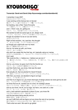
• If you know the price of certain stock from day
i to day j;
• You can only buy and sell one share once
• How to maximize your profit?
120
110
Price
100
90
80
70
60
0
1
2
3
4
5
6
7
8
day #
9
10
11
12
13
14
15
16
Maximum-Subarray Example
Example:
Maximum-Subarray Example
Buying low and selling high doesn’t always work
Best strategy:
Buy here
Sell here
But doesn’t
follow “buy low,
sell high” rule
Maximum-subarray problem
• What is the brute-force solution?
max = -infinity;
for each day pair p {
if(p.priceDifference>max)
max=p.priceDifference;
}
Time complexity?
Maximum-subarray problem
• What is the brute-force solution?
max = -infinity;
for each day pair p {
if(p.priceDifference>max)
max=p.priceDifference;
}
Time complexity?
𝑛
2
pairs, so O(𝑛2 )
How to solve more efficiently?
• If we know the price difference of each 2
contiguous days
• The solution can be found from the
maximum-subarray
• Maximum-subarray of array A is:
– A subarray of A
– Nonempty
– Contiguous
– Whose values have the largest sum
Examine subarrays
Day
Price
Difference
0
10
1
11
1
2
7
-4
3
10
3
4
6
-4
Remember best solution: Buy on day 2, sell on day 3
Examine the differences across subarrays (some examples):
Sub-array
Difference
0-1
1
0-2
-3
0-3
0
0-4
-4
2-2
-4
2-3
-1
2-4
-5
3-3
3
3-4
-1
4-4
-4
Divide-and-Conquer Approach
• How to divide?
– Divide into 2 arrays
• What is the base case?
• How to combine the subproblem solutions?
Divide-and-Conquer Approach
• Note where solution must lie:
• 3 choices:
– A[i, …, mid] // best is in the left array
– A[mid+1, …, j] // best is in the right array
– A[ …, mid, mid+1….] // best is in the array across the midpoint
– The maximum subarray for A[i,…,j] is the best of
these 3 choices
Maximum-subarray problem – divideand-conquer algorithm
Input: array A[i, …, j]
Ouput: sum of maximum-subarray, start point of maximum-subarray,
end point of maximum-subarray
FindMaxSubarray:
1. if(j<=i) return (A[i], i, j);
2. mid = floor(i+j);
3. (sumCross, startCross, endCross) =
FindMaxCrossingSubarray(A, i, j, mid);
4. (sumLeft, startLeft, endLeft) = FindMaxSubarray(A, i, mid);
5. (sumRight, startRight, endRight) = FindMaxSubarray(A, mid+1, j);
6. Return the largest of these 3
Maximum-subarray problem – divideand-conquer algorithm
Input: array A[i, …, j]
Ouput: sum of maximum-subarray, start point of maximum-subarray,
end point of maximum-subarray
FindMaxSubarray:
1. if(j<=i) return (A[i], i, j);
2. mid = floor(i+j);
3. (sumCross, startCross, endCross) =
FindMaxCrossingSubarray(A, i, j, mid);
4. (sumLeft, startLeft, endLeft) = FindMaxSubarray(A, i, mid);
5. (sumRight, startRight, endRight) = FindMaxSubarray(A, mid+1, j);
6. Return the largest of these 3
Time complexity?
Maximum-subarray problem – divideand-conquer algorithm
Input: array A[i, …, j]
Ouput: sum of maximum-subarray, start point of maximum-subarray,
end point of maximum-subarray
FindMaxSubarray:
1. if(j<=i) return (A[i], i, j);
2. mid = floor(i+j);
3. (sumCross, startCross, endCross) =
FindMaxCrossingSubarray(A, i, j, mid);
4. (sumLeft, startLeft, endLeft) = FindMaxSubarray(A, i, mid);
5. (sumRight, startRight, endRight) = FindMaxSubarray(A, mid+1, j);
6. Return the largest of these 3
Time complexity?
𝑇 𝑛 = 2𝑇
𝑛
2
+ Θ(n)
Maximum-subarray problem – divideand-conquer algorithm
Input: array A[i, …, j]
Ouput: sum of maximum-subarray, start point of maximum-subarray,
end point of maximum-subarray
FindMaxSubarray:
1. if(j<=i) return (A[i], i, j);
2. mid = floor(i+j);
3. (sumCross, startCross, endCross) =
FindMaxCrossingSubarray(A, i, j, mid);
4. (sumLeft, startLeft, endLeft) = FindMaxSubarray(A, i, mid);
5. (sumRight, startRight, endRight) = FindMaxSubarray(A, mid+1, j);
6. Return the largest of these 3
Time complexity?
𝑇 𝑛 = 2𝑇
𝑛
2
+ Θ(n) = Θ(n lg n)
In-Class Exercise for Divide & Conquer
• Suppose you are given a complete binary tree of height h with n = 2h
leaves. [Here, we'll assume that the tree is completely filled in at all
levels, including the deepest level.]
• Each node and each leaf, x, in the tree has an associated "value" v(x),
which is an arbitrary real number.
• If x is a leaf, we denote by A(x) the set of ancestors of x (including x as
one of its own ancestors). That is, A(x) consists of x, x's parent,
grandparent, etc., up to the root of the tree.
• Let f(x) be the sum of the values of A(x) – that is, 𝑓 𝑥 = ∑𝑦∈𝐴(𝑥) 𝑣(𝑦).
• Presume we have the functions left(x), right(x), and parent(x), which
return pointers to the left child, right child, and parent of node x,
respectively. These functions return nil when no such node exists.
Give an efficient algorithm that finds the maximum value of f(x) across
all leaves x of the tree. Note that we do not need to know which set of
ancestors, A(x), sums to this maximum total; we only need to know its
value.
Dynamic Programming
• Dynamic programming is typically applied to
optimization problems. In such problem there
can be many solutions. Each solution has a
value, and we wish to find a solution with the
optimal value.
Optimization
This, generally, refers to classes of problems that possess multiple
solutions at one level, and where we have a real-valued function
defined on the solutions.
Problem: find a solution that minimizes or maximizes the value of
this function.
Note: there is no guarantee that such a solution will be unique
and, moreover, there is no guarantee that you will find it (local
maxima) unless the search is over a small enough search space or
the function is restricted enough.
Optimization
Question: are there classes of problems for which you can
guarantee an optimizing solution can be found?
Optimization
Question: are there classes of problems for which you can
guarantee an optimizing solution can be found?
Answer: yes. BUT you also need to find such a solution in a
"reasonable" amount of time.
We are going to look at two classes of problems, and the
techniques that will succeed in constructing their solutions in a
"reasonable" (i.e., low degree polynomial in the size of the initial
data) amount of time.
Optimization
We begin with a rough comparison that contrasts a method you
are familiar with (divide and conquer) and the method (still
unspecified) of Dynamic Programming (developed by Richard
Bellman in the late 1940's and early 1950's).
Two Algorithmic Models:
Divide &
Conquer
Dynamic
Programming
View problem as collection of
subproblems
“Recursive” in nature
Independent subproblems
Overlapping subproblems
Number of subproblems
depends on
partitioning
factors
typically small
Preprocessing
characteristic running time
Typically log
function of n
depends on number
and difficulty of
subproblems
Primarily for optimization
problems
Optimal substructure:
optimal solution to problem
contains within it optimal
solutions to subproblems
The Primary Steps of Dynamic Programming
1. Characterize the structure of an optimal solution.
2. Recursively define the value of an optimal solution.
3. Compute the value of an optimal solution in a bottom
up fashion.
4. Construct an optimal solution from computed
information.
Example: Rod Cutting
• You are given a rod of length n ≥ 0 (n in inches)
• A rod of length i inches will be sold for pi dollars
• Cutting is free (simplifying assumption)
• Problem: given a table of prices pi determine the
maximum revenue rn obtainable by cutting up the rod
and selling the pieces.
Length i
Price pi
1
1
2
5
3
8
4
9
5 6 7 8 9 10
10 17 17 20 24 30
Example: Rod Cutting
We can see immediately (from the values in the table) that
n ≤ pn ≤ 3n.
This is not very useful because:
• The range of potential revenues is very large
• Our finding quick upper and lower bounds depends on
finding quickly the minimum and maximum pi/i ratios
(one pass through the table), but then we are back to the
point above….
Example: Rod Cutting
Step 1: Characterizing an Optimal Solution
Question: in how many different ways can we cut a rod of length n?
For a rod of length 4:
Example: Rod Cutting
Step 1: Characterizing an Optimal Solution
Question: in how many different ways can we cut a rod of length n?
For a rod of length 4:
Options: 24 - 1 = 23 = 8
For a rod of length n: 2n-1. Exponential: we cannot try all possibilities for n "large".
The obvious exhaustive approach won't work.
Example: Rod Cutting
Step 1: Characterizing an Optimal Solution
Question: in how many different ways can we cut a rod of length n?
Proof Details: a rod of length n can have exactly n-1 possible cut positions –
choose 0 ≤ k ≤ n-1 actual cuts. We can choose the k cuts (without repetition)
anywhere we want, so that for each such k the number of different choices is
 n −1


 k 
When we sum up over all possibilities (k = 0 to k = n-1):
 n −1
n−1
(n −1)!
∑k= 0 k  = ∑k= 0 k!(n −1− k)! = (1+ 1)n−1 = 2n−1.
n−1
For a rod of length n: 2n-1.
Example: Rod Cutting
Characterizing an Optimal Solution
Let us find a way to solve the problem recursively (we might be able to
modify the solution so that the maximum can be actually computed):
Assume we have cut a rod of length n into 0 ≤ k ≤ n pieces of length i1, …, ik,
n = i1 +…+ ik,
with revenue:
rn = pi1 + … + pik
Assume further that this solution is optimal.
How can we construct it?
Advice: when you don’t know what to do next, start with a simple example
and hope something will occur to you… 
Example: Rod Cutting
Characterizing an Optimal Solution
Length i
Price pi
1
1
2
5
3
8
4
9
5 6 7 8 9 10
10 17 17 20 24 30
We begin by constructing (by hand) the optimal solutions for i = 1, …, 10:
r1 = 1 from soln. 1 = 1 (no cuts)
r2 = 5 from soln. 2 = 2 (no cuts)
r3 = 8 from soln. 3 = 3 (no cuts)
r4 = 10 from soln. 4 = 2 + 2
r5 = 13 from soln. 5 = 2 + 3
r6 = 17 from soln. 6 = 6 (no cuts)
r7 = 18 from soln. 7 = 1 + 6 or 7 = 2 + 2 + 3
r8 = 22 from soln. 8 = 2 + 6
r9 = 25 from soln. 9 = 3 + 6
r10 = 30 from soln. 10 = 10 (no cuts)
Example: Rod Cutting
Characterizing an Optimal Solution
Notice that in some cases rn = pn, while in other cases the optimal revenue rn is
obtained by cutting the rod into smaller pieces.
In ALL cases we have the recursion
rn = max(pn, r1 + rn-1, r2 + rn-2, …, rn-1 + r1)
exhibiting optimal substructure
A slightly different way of stating the same recursion, which avoids repeating some
computations, is
rn = max1≤i≤n(pi + rn-i)
This latter relation can be
implemented as a simple top-down
recursive procedure:
Example: Rod Cutting
Characterizing an Optimal Solution
Time Out: How to justify the step from:
rn = max(pn, r1 + rn-1, r2 + rn-2, …, rn-1 + r1)
to
rn = max1≤i≤n(pi + rn-i)
Note: every optimal partitioning of a rod of length n has a first cut – a segment of,
say, length i. The optimal revenue, rn, must satisfy rn = pi + rn-i, where rn-i is the
optimal revenue for a rod of length n – i. If the latter were not the case, there
would be a better partitioning for a rod of length n – i, giving a revenue r’n–i > rn-i
and a total revenue r’n = pn + r’n-i > pi + rn-i = rn.
Since we do not know which one of the leftmost cut positions provides the largest
revenue, we just maximize over all the possible first cut positions.
Example: Rod Cutting
Characterizing an Optimal Solution
We can also notice that all the items we choose the maximum of are
optimal in their own right: each substructure (max revenue for rods
of lengths 1, …, n-1) is also optimal (again, optimal substructure
property).
Nevertheless, we are still in trouble: computing the recursion leads
to recomputing a number (= overlapping subproblems) of values –
how many?
Example: Rod Cutting
Characterizing an Optimal Solution
Let’s call Cut-Rod(p, 4), to see the effects on a simple case:
The number of nodes for a tree corresponding to a rod of size n is:
T (0) = 1,
T(n) = 1+ ∑
n−1
j= 0
T( j) = 2 n , n ≥ 1.
Example: Rod Cutting
Beyond Naïve Time Complexity
We have a problem: “reasonable size” problems are not solvable in
“reasonable time” (but, in this case, they are solvable in “reasonable
space”).
Specifically:
• Note that navigating the whole tree requires 2n work.
• Note also that no more than n + 1 subproblems are active at any one time
and that no more than n + 1 different values need to be computed or used.
Can we exploit these observations?
A standard solution method involves saving the values associated with
each T(j), so that we compute each value only once (called “memoizing” =
writing yourself a memo).
Example: Rod Cutting
Naïve Caching
We introduce two procedures:
Example: Rod Cutting
More Sophisticated Caching By Solving Bottom-Up
Example: Rod Cutting
Time Complexity
Whether we solve the problem in a top-down or bottom-up manner
the asymptotic time is Θ(n2), the major difference being recursive
calls as compared to loop iterations.
Why??
Handy Tool: Subproblem graphs
• For rod-cutting problem with n = 4
– Subprogram graph is a directed graph
• One vertex for each distinct
subproblem.
• Has a directed edge (x, y) if
computing an optimal solution to
subproblem x directly requires
knowing an optimal solution to
subproblem y.
Subproblem graphs
• Can think of the subproblem graph as a collapsed
version of the tree of recursive calls, where all nodes
for the same subproblem are collapsed into a single
vertex, and all edges go from parent to child.
• Subproblem graph can help determine running time.
Because we solve each subproblem just once, running
time is sum of times needed to solve each subproblem.
– Time to compute solution to a subproblem is typically
linear in the out-degree (number of outgoing edges) of its
vertex.
– Number of subproblems equals number of vertices.
• When these conditions hold, running time is linear in
number of vertices and edges.
Reconstructing a solution
• So far, have focused on computing the value
of an optimal solution, rather than the choices
that produced an optimal solution.
• Extend the bottom-up approach to record not
just optimal values, but optimal choices. Save
the optimal choices in a separate table. Then
use a separate procedure to print the optimal
choices.
Reconstructing a solution
Reconstructing a solution
In-Class Exercise
• Draw the recursion tree for the MERGE-SORT
procedure on an array of 16 elements. (Each node of
the recursion tree should simply indicate which
elements of the array are being solved at that node.)
• Explain why memoization is ineffective in speeding
up a good divide-and-conquer algorithm such as
MERGE-SORT.
The Primary Steps of Dynamic Programming
1. Characterize the structure of an optimal solution.
2. Recursively define the value of an optimal solution.
3. Compute the value of an optimal solution in a bottom
up fashion.
4. Construct an optimal solution from computed
information.
Reading Assignments
• Today’s class:
– Chapter 4.1, 15.1
• Reading assignment for next class:
– Chapter 15.2 (Matrix chain multiplication)

Download Report