URSI-France Journées scientifiques 25/26 mars 2014 Statistical Simulations of a Body-Worn Triaxial Sensor for Electromagnetic Field and Exposure Assessment Christophe Roblin* *LTCI, Télécom ParisTech & CNRS, Paris, France, [email protected] Key words EMF exposure, exposimeter, exposure index, field sensor. Introduction The Electromagnetic Field (EMF) exposure of the population due to wireless communications (2G, 3G, 4G and WLANs) originates both from Down-Link (DL) emissions incoming from Base Stations (BS) and Access Points (AP), and from Up-Link ones produced by the terminals (cell phones, tablets and lap-tops). Although the main contribution comes generally from the last, the former must be considered as well, as contributions can be competitive for some cases for which both (e.g. in femtocells. Note however that in this case, the EMF levels are particularly low. In any case, DL emissions are continuous whereas UL ones are time limited. One of the main objectives of the EU FP7 project Lexnet is to propose innovative technical solutions to reduce the exposure level of the population, in a global way, without affecting quality of service. The possible improvements are investigated in every parts of the system, both in terms of technology (antennas, sensitivity, wake-up strategy, RRM, power control, etc.) and in terms of architectures and network (NW) management (heterogeneous networks, offloading, densification, etc.). To this end, a new Exposure Index (EI) merging both UL and DL emissions is defined, noting notably that, up to now, the exposure sources have been considered separately with different “metrics” (the SAR for the UL one and the field level for the DL one). The EI aggregates all sources of exposure due to wireless networks (excluding broadcasting, power lines and all other sources) operating in a given area: it takes into account the environment (type of area –urban to rural– and location –indoor, outdoor), the population present in the considered area (apportioned according to several user profiles), the time of day (traffic loading), the NW RATs (2G, 3G, etc.) and layers (macro to femto cells), and terminals usages (voice, data modes, user posture). The EI is inherently an average quantity assessed statistically. The Near Field (NF) contribution (UL) is estimated thanks to SAR simulations for various models of sources (terminals) and users (numerical phantoms). The DL contribution is obtained from the assessment of the whole body SAR induced by BSs or the APs for each considered configurations. For the last, the SAR evaluation is related to the field strength at which the user is exposed. This field level can be estimated in different ways: first, through the NW to which the user is connected, second, thanks to information collected by disseminated field sensors or personal dosimeters directly worn by some users (called exposimeters). Information known by a NW are available at BSs or APs (individual user device transmitted (Tx) and received (Rx) powers, BS or AP Tx power and traffic load) and can be profitably used, although they don’t aggregate heterogeneous data (ignoring e.g. emissions from other NWs) and are hence partial. With some software modifications or resorting to dedicated applications, Tx and Rx powers of some devices could be also known at their level, recorded and transmitted to the NW for recording and appropriate processing (notably statistical). Note that sensor and exposimeter NW can be deployed by the operators themselves or by independent external stakeholders such as regulatory agencies or local authorities. Besides these external actors, exposimeters are not only useful for a NW as they can bring complementary information about users, but also because they can provide information about their carriers who are not users or who are not currently using their devices. This paper addresses the issue of the field level assessment and more specifically its evaluation with exposimeters. The main technical challenge resides in the modeling of the measurement errors of body-worn sensors induced by proximity effects, notably the masking effect of the body. The results presented in section 2 are based on electromagnetic (e.m.) simulations briefly presented in section 1. A comprehensive measurement campaign was carried out with a triaxial sensor attached at three different locations on a whole body phantom. Measurements details are presented in section 1 and preliminary results and discussion in section 2. 1. Approach and objectives As a first approach, a simulation of a simplified model (provided by Satimo ®) of the sensor of the EME Spy 140® dosimeter (from the company Satimo®) “worn” by a numerical phantom of the Virtual Population suit (from ITI’S foundation) [1]. The purpose of this preliminary analysis being to identify trends through statistical assessments, a 145 Journées scientifiques 25/26 mars 2014 URSI-France “small” phantom (“Eartha”, an 8-years old child girl) have been chosen in order to minimize the simulation time. The sensor is placed at a few millimeters of her chest (Fig. 1). The objectives of the article are: • To characterize the isolated sensor “isotropy” and its (significant) degradation induced by the body proximity, • To analyze the influence of the sensor probes’ polarization purity via the cross-polarization ratios (XPRP), • To analyze the influence of the depolarization effects induced on the one hand by the propagation channel (via the field XPR, XPRE), and on the other hand by the proximity of the body, • To show that, more generally, the characteristics of the propagation channel must be taken into account to correctly assess the sensor isotropy (or deviation to isotropy). For that purpose, three successive approaches are considered: • A polarimetric analysis of the isotropy (and a characterization of the XPRP), • A non polarimetric approach (combining all probes signals) allowing to characterize the influence of the incoming field XPR (XPRE), • And a non polarimetric statistical analysis accounting for the propagation channel properties (notably its 3D angular spectrum and polarization characteristics). The antenna transfer function (ATF) H ( f,,) [1] is computed (either in the transmitting or receiving mode) from the Far Field calculated over 0.5 – 6 GHz by the Time Domain solver of CST Microwave Studio®, for each axial probe and possible configuration (only one is considered here). The definition used for the ATFs is recalled hereafter for clarity: En ( f , rˆ ) e jkr r bn ( f , rˆ ) e jk i r 0 T H n ( f , rˆ ) an 4 4 0 H nR ( f , rˆ ) Ei (k i , r) 1 4 c T j H n ( f , rˆ ) Ei 0 2 0 where an (resp. bn) is the incident (the received) wave at the n-th probe port, H R (resp. H T ) is the antenna transfer functions in the receiving (resp. transmitting) modes, 0 thee free space impedance, the angular frequency, k the wavenumber, En the radiated Far Field (FF), ki the wave vector of the incident plane wave Ei and Ei0 = Ei( f,0) denotes the z field at the origin chosen at the center of the sensor spherical ground. A priori, apart from a frequency scaling, the directional and polarization characteristics are the same in both x y modes. The reflection coefficients S11 at each probe port are also computed for each considered configuration. All relevant quantities (realized gain Gr, radiation or total Fig. 1. Sketch of the triaxial efficiencies and (loaded) antenna factor AF ) can be computed from the ATF, for each sensor placed on Eartha’s polarization. Each component of the radiated FF, or its magnitude, can be computed as phantom chest well for a given incident power density. These characteristics are presented for both isolated and worn sensor, for the main communication bands (GSM900, GSM1800, UMTS, LTE800 & 2600, and WiFi 2.45 GHz 5.5 GHz) ; the results are averaged over each frequency band. 2. Preliminary Results 2.1. Triaxial isolated and body-worn sensor main characteristics – polarimetric approach The main directional characteristics of the sensor are presented in the following figures. The “isotropy” of the isolated sensor is very satisfactory, in particular for the “H” probes, with standard deviations G ranging typically between 1 and 3 dB. The sensor XPR is very satisfactory for the “V” probe over a wide solid angle around the horizon (typ. less than 10 dB). It is a little bit higher for the H probes in particular for the lower frequency bands (typ < 5 dB), in agreement with the measurements (not considered in this paper). The results are, as expected, completely different for the worn sensor, the shadowing effect of the body being dominant. Standard deviations of the realized gain (relative to the isolated one in the azimuthal plane) are typically in the range Gv ~ 7 – 10 dB (V probe) and Gh ~ 2.5 – 6.5 dB (H probes), with FTBR (Front To Back ratios) as high as 30 dB. In addition, the body proximity induces a significant degradation notably of the V probe XPR (by 2 to 16 dB on average, depending on the band), which is not surprising as it is tangent to the body (which favors energy coupling). In the following, the realized gains (and all the other considered quantities) are normalized to that of the isolated sensor (in the azimuth plane) in order to focus on the isotropy variance and polarization aspects, and to underline the body effect. All the considered moments (expectations and variances) are related to these normalized quantities: 2 1 Gˆ r,,phant ( f RAT , , ) = Gr,,phant ( f , , ) df / Gr,,isol ( f , / 2, ) d df 0 2 f RAT f RAT 2.2. Non polarimetric approach As the polarization of the incoming wave is a priori not known on the one hand, and, in the other hand, as the sensor XPR is not always low as abovementioned, a non polarimetric approach is presented hereafter. The influence of the incoming wave XPR is first considered. For simplicity, the analysis is restricted to linear polarization. To this end, the sensor is analyzed in the receiving mode instead of in the transmitting mode as previously. 146 URSI-France Journées scientifiques 25/26 mars 2014 -20 0 2 0 0 0 0 -2 180 -25 180 180 -30 270 270 -8 270 -6 -8 -10 90 90 -40 -10 90 -12 -12 -14 0 0 LTE 2600 WiFi 5G -18 180 -16 180 0 0 -14 0 -16 -45 LTE 800 -4 -6 -35 180 -2 -4 0 2 -20 2 1 -21 270 270 0 180 180 0 270 180 -1 -22 -2 -2 -4 -23 -3 0 LTE 800 180 -5 -25 90 -6 -4 -24 0 90 -26 180 0 -8 90 -6 LTE 2600 -10 WiFi 5G -7 180 Fig. 1. Isolated sensor. Simulated 3D co-polar realized gain patterns (averaged over each RAT band, LTE 800, LTE 2600 and WiFi 5G) of the (top) “V”(z’Oz) probe (-polarization) and (bottom) combined “H” (xOy) probes (-polarization). 270 0 270 -20 5 270 0 0 0 180 180 -5 180 -25 0 -5 0 -30 -10 -35 0 -15 0 -10 180 180 180 -40 3D Realized gain patterns - GSM 900 z'Oz probe, V polarization -20 90 90 3D Realized gain patterns - LTE 2600 z'Oz probe, V polarization -45 3D Realized gain patterns - WiFi 5G z'Oz probe, V polarization -25 5 270 -20 0 180 270 0 0 -22 0 0 180 180 -5 -5 -24 -26 -10 -10 -28 0 0 0 -30 180 90 3D Realized gain patterns - GSM 900 combined x'Ox & y'Oy probe, H polarization -15 -15 180 180 90 90 -32 -34 -20 5 -18 270 -15 90 3D Realized gain patterns - LTE 2600 combined x'Ox & y'Oy probe, H polarization -20 -20 3D Realized gain patterns - WiFi 5G combined x'Ox & y'Oy probe, H polarization Fig. 2. Body-worn sensor. Simulated 3D co-polar realized gain patterns (averaged over each RAT band, GSM 900, LTE 2600 and WiFi 5G) of (top) the “V”(z’Oz) probe (-polarization) and (bottom) combined “H” (xOy) probes (-polarization). H ˆ The XPR of the incident plane wave Ei 0 EiV0 θˆ EiH 0 φ is defined as xprE Ei 0 2 / EiV0 2 and the field strength is set to 1 V/m, so that: EiV0 1 (1 xprE )1/2 and Ei 0H xprE1/2 (1 xprE )1/2 expressed in V/m. Note that, besides the field component amplitude, the signs (i.e. the phase) of these components is important, as the field can be in any quadrant of any plane tangent to the sphere, and as the probes are not purely polarized, so that each projection must be added at the field level and not in power. 147 Journées scientifiques 25/26 mars 2014 URSI-France The XPR is expressed in dB in the sequel, i.e. : XPRE = 10 log xprE. The received signal b is computed as a normalized combination of the signals received at each probe port, i.e.: b bv2 bh2 1/2 bv2 ( f RAT , , xpr ) with: 2 f RAT H z Ei 0 df f RAT H z ,isol 2 and bh2 ( f RAT df , , xpr ) f RAT 2 2 f RAT H x Ei 0 H y Ei 0 df 2 H x,isol H y ,isol 2 df where x, y (resp. z) refer to the “H” probes (resp. “V” probe), <·> denotes an averaging over variable , and the superscript “T” has been omitted in the ATF notation to ease the readability (actually any of the Tx or Rx ATF can be used in these expressions). It is easy to show that b 1 for an “ideal” sensor, i.e. perfectly matched, lossless and fully isotropic. As expected, the isotropy is improved when we resort to a non polarimetric received signal (combining all probes’ signals), including for the isolated sensor (although slightly, typ. by less than 1 dB for b compared to Gv), as can be observed in the following figures and table. The counterparty is of course that the polarization information is not anymore used (and lost in b ), although signals of each probe are still available and could be exploited besides. Non polarimetric isotropy (all axes) Standard deviation over AoA (dB) - all Non polarimetric isotropy (all axes) Standard deviation over azimuth (dB) - UMTS band (integrated over 1.9 - 2.15 GHz) 8 9 7 8 GSM 900 GSM 1800 7 6 10 (dB) LTE 800 5 (dB) UMTS 6 5 4 20 WiFi 2G WiFi 5G 4 3 10 0 200 LTE 2600 5 3 2 0 150 (°) 100 -10 50 0 XPRv2h (dB) V polar 1 2 -20 -15 -10 H polar -5 0 5 10 15 20 XPRv2h (dB) -20 Fig. 3. Influence of the incoming wave XPR on the non polarimetric received signal b . Left: example including the dependence (UMTS band). As can be seen in Fig. 3, the influence of XPRE is significant and should be consequently taken into account. There is actually an “interaction” between XPRE and XPRP. On average, as can been seen in Table 1, the variance of the non polarimetric signal is reduced compared to that of the “V” probe. This is interesting as, on the one hand, most of the RATs transmit in V polarization, and on the other hand, typical values of XPRE range between 15 and 5 dB, depending on the propagation channel depolarization properties, i.e. on the environment (Macrocell, Indoor, LOS, NLOS, etc.). The measurement “biases”, which actually correspond to the averages of the same quantities (not shown here for brevity) are also reduced when using the non polarimetric signal instead of the polarimetric ones. Note also that, both in Fig. 3 and Table 1, all the elevations are considered so that the variances of b are overestimated compared to what would be obtained with realistic elevation spreads encountered in practice (in real channels). In any case, it appears here that the channel characteristics must be accounted for to correctly assess the reliability of the sensor measurement. This is the object of the last part of this section (as a really preliminary study). The received signal b is computed in the same way as before (in the non polarimetric deterministic analysis), but the field obeys now the statistical laws of the channel model. The total field level is still fixed to Ei0 = 1 V/m, but its energy is angularly spread in several “clusters” considered here for simplification as simple Multi Path Components (MPCs). The PL modelling is irrelevant here as we are dealing with received waves and not radio link budgets. In the same way, the delay domain is not of concern as the signal is integrated at the receiver over durations which are far larger than the delay spread. The carrier phase aspect, and related small scale (or selective) fading is neither considered in order to simplify the approach, and also, more fundamentally, because in practice measurements are averaged over time and/or space. The environment type (“scenarios” in WINNER [3], [4] models such as Indoor, Outdoor to Indoor (O2I), Urban Macrocells (UMa), in LOS or NLOS, etc.), the number of clusters (MPCs), the angular spectrum (Angle of Arrival, AoA) and polarization statistics (XPR) are however taken into account. The elevation spread is based on the WINNER+ models [5]. In the simplified model which will be used, the number of paths, angular spectrum and XPR don’t depend explicitly on the frequency, although they depend on the environment which is, for some, related to the RATs frequency bands (i.e. WLANs are mainly used in indoor environments and over WiFi bands). In other words any explicit frequency dependence of these parameters is neglected here. Two environments – Office/room Indoor (NLOS) and UMa (LOS) – are considered as examples. The channel model details (structure and parameters) are not given here due to lack of space. 148 URSI-France Journées scientifiques 25/26 mars 2014 For the isolated sensor, there is almost no bias in the field assessment for all the LOS scenarios and almost all NLOS scenarios (means are very close to 1 V/m). On the other hand, in all cases, as can be observed in Tables 1, the variance is significantly higher than those of the deterministic analyses (polarimetric or not), ranging between 4 and 6 dB (instead of 1 – 2.5 dB). It is of course due to the fact that the channel characteristics were not previously taken into account: in particular, there is an interaction between the probes XPR and the channel depolarization effect, and above all, the signal received by each probe is a linear combination of signals proportional to the field of each MPC which consequently involves not only the directional amplitude variation of their transfer functions, but also their polarity variation. Note that if the same computations are performed with an hypothetic channel characterized by a small number of MPCs and a small angular spread, we find back results similar to those of the deterministic non polarimetric analysis. For the body-worn sensor, the variance is larger than that of the deterministic approach for the same reasons, but smaller than that of the -polarization component of the “V” probe (and slightly larger than the -polarization component of the “H” probes). We attribute this result to the “isotropization” effect of the combined non polarimetric signal. Table 1 : Measurement and simulation approaches summary: standard deviations. Isolated sensor Detection Body-worn sensor Ei0 Gv Gh bV bH b 1.35 4.3/4.0 7.0 3.0 4.4 2.8 3.4 4.4/5.7 1.5 1.4 4.2/3.9 9.4 5.0 7.1 4.8 5.9 6.6/9.2 0.9 1.6 1.2 4.2/3.9 9.6 5.7 7.4 5.6 6.4 7.2/9.7 1.5 2.1 1.7 4.0/3.9 10.2 6.6 7.9 6.3 7.0 7.3/9.7 dispersion Gv Gh bV bH b GSM 900 2.5 1.0 1.4 1.3 UMTS 2.6 1.2 1.3 LTE 2600 2.0 1.2 WiFi 5G 1.9 1.9 Env. n° 1/2 Ei0 Env. n° 1/2 2.3. Possible correction Strategies Recently, it has been proposed in [6] to resort to several exposimeters (in this case at 950 MHz) to compensate for the shadowing and reflection effects, and somehow “regain” omnidirectionality. The results improvement of this interesting approach is really significant. However, although the system uses textile antennas and wearable electronics, one wonder if it can be easily used on a large scale, in particular with regard to its user acceptability, or if it will be restricted to professionals. Various other approaches [7], [8] have been proposed in the literature, in particular based on daily activity recording. Data fusion, resorting notably to compact inertial units signals, aided or not with a GPS signal, are promising. 3. Conclusions The presented results confirm that the dispersion of measurements collected by exposimeters is large. It shows that resorting to a non polarimetric combined signal tends to improve the isotropy, but that taking account of the propagation channel is mandatory in order to correctly assess the field measurement reliability. Anyway, corrections schemes are required to overcome the body shadowing effect which is dominant. This aspect will be thoroughly studied in future works. To complete these first results, a comprehensive simulation campaign is on-going in the framework of the Lexnet project. Its objective is to take into account other significant parameters such as anthropometric characteristics (size, corpulence, or BMI), as it is expected that their impact on shadowing effects would be significant. Acknowledgment Authors would like to thank SATIMO for providing the dosimeter numerical model and Alain Sibille for fruitful discussions and his kind help in providing Matlab routines for the simulation of the propagation channel (based on WINNER+ models). This paper reports work undertaken in the context of the project LEXNET. LEXNET is a project supported by the European Commission in the 7th Framework Programme (GA n°318273). For further information, please visit www.lexnet-project.eu. References [1] [2] [3] [4] [5] [6] [7] [8] http://www.itis.ethz.ch/itis-for-health/virtual-population/human-models/ C. Roblin, S. Bories, and A. Sibille, “Characterization tools of antennas in the Time Domain,” IWUWBS, Oulu, June 2003. J. Meinilä, T. Jämsä, P. Kyösti, D. Laselva, H. El-Sallabi, J. Salo, C. Schneider, D. Baum, “D5.2, Determination of Propagation Scenarios,” IST-2003-507581 WINNER, 16/07/2004. Pekka Kyösti, Juha Meinilä, Lassi Hentilä, Xiongwen Zhao, Tommi, Jämsä, Christian Schneider, Milan Narandzić, Marko Milojević, Aihua Hong, Juha Ylitalo, Veli-Matti Holappa, Mikko Alatossava, Robert Bultitude, Yvo deJong, Terhi Rautiainen, “D1.1.1 V1.1, WINNER II interim channel models,” IST-4-027756 WINNER II, 30/11/2006. Juha Meinilä, Pekka Kyösti, Lassi Hentilä, Tommi Jämsä, Essi Suikkanen, Esa Kunnari, Milan Narandžić, “D5.3: WINNER+ Final Channel Models,” WINNER+, CELTIC / CP5-026, 30.6.2010 A. Thielens et al, “Design and Calibration of a Personal, Distributed Exposimeter for Radio Frequency Electromagnetic Field Assessment,” COST IC1004, TD(13)08033, Ghent, Belgium, 25-27 Sept. 2013. J. Blas et al, “Potential exposure assessment errors associated with body-worn RF dosimeters,” Bio Electro Magnetics, 28(7), 2007. S. Iskra et al, “Factors influencing uncertainty in measurement of electric fields close to the body in personal RF dosimetry,” Radiation Protection Dosimetry, 140(1), 2010. 149
© Copyright 2026 ExpyDoc