ECE455, Optional Experiment, 2014
Communications Lab, University of Toronto
Optional Experiment: Instruments and Workstation
Bruno Korst - [email protected]
Abstract
In this optional experiment, you will review some aspects of the instruments and tools used in this course, and will
run a black-box system to find out what it does. For this course, most experiments are simulated on Simulink
and implemented on a DSP platform. This outline will also serve as a guide to Simulink and Code Composer
Studio if you need one in the future.
Keywords
Oscilloscope — Signal Generator — Fourier Series — Sinusoid — Square Wave — Simulink — Time Domain
Scope — Frequency Domain Scope — Code Composer Studio
Contents
Introduction
1
1
Suggested Reading
2
2
Equipment and Software Tools
2
3
The Instruments
2
3.1 The Tektronix AFG3021 . . . . . . . . . . . . . . . . . . . . . . . . . . . . . . . . . . . . . . . . . . . . . . . . . . . . . . . . . . . . . 2
3.2 The Tektronix TDS 2012 Oscilloscope . . . . . . . . . . . . . . . . . . . . . . . . . . . . . . . . . . . . . . . . . . . . . . . . . . . 3
The Trigger • The Math/FFT Function • Cursors • The Measure Feature
4
Some Practice...
4
4.1 With a Sine Wave and the Oscilloscope . . . . . . . . . . . . . . . . . . . . . . . . . . . . . . . . . . . . . . . . . . . . . . . . . . 5
4.2 With a Pulse and the Oscilloscope . . . . . . . . . . . . . . . . . . . . . . . . . . . . . . . . . . . . . . . . . . . . . . . . . . . . . 5
5
Introduction to Matlab and Simulink
5.1
5.2
5.3
5.4
Simulating a Scope . . . . . . . . .
Simulating a Spectrum Analyzer
Simulating a Square Wave . . . .
Adding Multiple Sinusoids . . . . .
6
Introduction to Code Composer Studio v5.4
.
.
.
.
.
.
.
.
.
.
.
.
6
.
.
.
.
.
.
.
.
.
.
.
.
.
.
.
.
.
.
.
.
.
.
.
.
.
.
.
.
.
.
.
.
.
.
.
.
.
.
.
.
.
.
.
.
.
.
.
.
.
.
.
.
.
.
.
.
.
.
.
.
.
.
.
.
.
.
.
.
.
.
.
.
.
.
.
.
.
.
.
.
.
.
.
.
.
.
.
.
.
.
.
.
.
.
.
.
.
.
.
.
.
.
.
.
.
.
.
.
.
.
.
.
.
.
.
.
.
.
.
.
.
.
.
.
.
.
.
.
.
.
.
.
.
.
.
.
.
.
.
.
.
.
.
.
.
.
.
.
.
.
.
.
.
.
.
.
.
.
.
.
.
.
.
.
.
.
.
.
.
.
.
.
.
.
.
.
.
.
.
.
.
.
.
.
.
.
.
.
.
.
.
.
.
.
.
.
.
.
.
.
.
.
.
.
.6
.6
.7
.8
8
6.1 The Hardware . . . . . . . . . . . . . . . . . . . . . . . . . . . . . . . . . . . . . . . . . . . . . . . . . . . . . . . . . . . . . . . . . . . . 9
Exercises with the Hardware
7
Conclusion
10
Acknowledgments
10
References
10
Introduction
This experiment will have you run a series of exercises that are meant to prepare you for future experiments. All skills learned
and used here will be necessary for the experimental portion of the course.
We will start from the Oscilloscope and Signal generator, and will move on to the software packages that you will use,
Simulink and Code Composer Studio. These are tools widely used in both academia and the industry. The latter is used
Optional Experiment: Instruments and Workstation — 2/10
in this lab to program an TMDXLCDK138, platform, based on a dual-core ARM+DSP processor. This is one of the latest
family of processors from Texas Instruments.
For future experiments, it is a good idea to read the outline prior to the experiment in order to become familiar with the
diagrams and individual blocks that will be used. Needless to say, make sure the preparation is done as well.
1. Suggested Reading
You should prepare for this first experiment by reviewing Fourier Series from your Signals and Systems course. You must be
familiar with time domain / frequency domain representation of signals. You can review [1] or [2], for instance. For this exercise
session, you will be presented with very simple input-output block diagrams to demonstrate the capabilities of Simulink.
2. Equipment and Software Tools
The following list of equipment and software tools will be utilized in all experiments.
Hardware:
• One Signal Generator;
• One Two-Channel Oscilloscope;
• One TI LCDK DSP development platform attached to a PC workstation.
• Coaxial cables BNC-to-BNC and a T connector.
Software:
• Matlab 8.1 - Release 2013A;
• Simulink with DSP and Signal Processing Toolbox;
• Code Composer Studio (CCS), v.5.4.0.
3. The Instruments
Since you will implement your systems on a DSP platform, all your input signals from the signal generator will be presented to
an analog-to-digital converter prior to being processed by the DSP. The input of the converter is a high-impedance input. By
default, your signal generator assumes a 50Ω impedance at their output. This is to say that you must adjust the output of the
signal generators to “see” a large impedance. This is done by choosing a High Z output option, as described below.
In a similar fashion, the input to the oscilloscope – as a measuring device – is a very high impedance input. This is so to
prevent the instrument itself from interfering with the measurement being taken. The instrument must look like an open circuit
to the device under test. The very high (around 1MΩ) input impedance will accomplish this. There is no setting to be changed
on the oscilloscope.
3.1 The Tektronix AFG3021
In this lab you will use the Tektronix AFG3021. It is called arbitrary because it allows for waveforms to be designed and edited
either on the instrument or on a computer, and then loaded onto the instrument. Some of your experiments will utilize arbitrary
(i.e., made up) waveforms. Below are two settings which you will need throughout the course.
Turn the instrument on 1 . From the front panel, press Sine. You will see on the bottom right corner of your screen
a menu labeled Output Menu. Press on the corresponding button. Another menu will appear, in which you will find Load
Impedance. Press on it, and you will have three options. Select High Z. From this point on, your instrument is set to see a high
impedance load on its output. To return to the main screen, just press on Sine again.
Action
Make sure that the Output ON button is lit (if it is not, press it). It is located right above the BNC output connector.
Otherwise you will not have a signal. Note that the Output ON button is lit on Figure 1(a). When the output is ON, and the
output impedance is set to high, the message Load High Z will appear on the top right corner of the screen.
Action
1
it happens
Optional Experiment: Instruments and Workstation — 3/10
(a) Finding Output Menu (Output ON)
(b) Selecting High Z
Figure 1. Tektronix AFG 3021 - Output
3.2 The Tektronix TDS 2012 Oscilloscope
You may already be familiar with the oscilloscope (every Electrical Engineer should!), but it is good to review some features
that if not understood now will potentially cause you to waste precious time during the experiments. These are: the trigger, the
MATH/FFT function and the use of cursors for measuring voltage, time, amplitude and frequency. Just as a reminder, whenever
you are in the lab, try very hard to avoid pressing the Auto Set button. Yes, it is convenient and very popular, but you will not
learn as much about the instrument if you always use it. Students tend to assume that whatever is displayed after this button is
pressed must be the truth. Always read the numbers and see if they make sense. The trick is to know what to expect from the
instrument. The general rule is: if you understand what the Auto Set button does to get the readings, go ahead and use it.
3.2.1 The Trigger
In general, when you connect a signal source to your oscilloscope the signal ”runs” across your screen. In order for you to take
a reading, you should make it stop. The proper way to make it stop is to set up a voltage level at which the oscilloscope starts to
collect and display the signal. In other words, you should set up a trigger point. This is done by pressing the Trig Menu button
found at the right-most portion of your front panel, right under a rotating knob. As you press it, a soft menu appears on the right
side of the display. Select the trigger Source (i.e. channel 1 or 2 – we will not use any other), and a small arrow will appear
further to the right of the display. The colour of the arrow is the same as the channel chosen as the source. This arrow indicates
your trigger level. Rotate the knob that is over the Trig Menu button, and the arrow will move. Position the arrow within the
voltage span of your signal. This will make the signal stop on the display. Note that the signal continues to be collected and
displayed, but it is now steady on your display. If the signal changes in amplitude, frequency, or a feature appears, the display
will show it.
The improper way to make a signal stop is to press the Run/Stop button. In the exercise section of this document you will
do an exercise to understand why using Run/Stop will not be appropriate.
3.2.2 The Math/FFT Function
This scope allows you to see your signal in the frequency domain by means of an FFT operation. You can select the Math mode
by pressing a big fat red button right in the middle of the instrument.
Figure 2. Big Fat Red Button – Math Mode
Optional Experiment: Instruments and Workstation — 4/10
Figure 3 below shows you the time domain for two input channels and the corresponding frequency domain for one of those
channels. Both inputs are a 1KHz, 1Vpp sine wave.
(a) Time Domain: Two channels
(b) Frequency Domain: One Channel
Figure 3. Tektronix TDS 2012 Oscilloscope
After pressing the Math Menu button, you must select what type of operation you want the instrument to perform. For the
case of an FFT, you also must select the channel (Source) that you want to display. Figure 3(b) is showing the FFT mode for
Channel 1.
On FFT mode, the horizontal control works “opposite” to its time domain operation. This is to say that if you want to
”increase” the Hertz per Division reading you should turn the horizontal scale knob clockwise. In this case, what the instrument
is actually doing is selecting a different sampling rate for the input at every click of the horizontal scale knob. You should be
careful when using this knob to zoom in, as you may end up with aliasing depending on the type of signal you have (this will
likely happen in the exercise section below).
The proper way to zoom into the signal in the frequency domain is to use the FFT Zoom soft key. Note also that as you turn
the horizontal scale knob, at the bottom of the screen the number displayed changes, as it represents the horizontal scale units
of Hz per Division. Figure 3(b) shows the frequency component at 1KHz.
3.2.3 Cursors
In order for you to perform specific or relative measurements between points of a signal, the instrument allows you to place
cursors on the desired points, and presents you with the values at each cursor and the calculation for the difference between the
cursors. Cursors can measure differences in time (vertical cursors) and amplitude (horizontal cursors), or in Math mode they
can measure differences in magnitude and frequency. After pressing the cursors button on the top part of the front panel, you
will be presented with a menu to select the signal source (Channel 1, 2 or math) and the type of measurement you want.
3.2.4 The Measure Feature
The Measure button is found on the top part of the front panel. This feature is very convenient, but you should try to develop an
intuition whether the numbers displayed make sense. This usually comes with practice. For instance, if your measured output
from the DSP board is a 20 Vpp sine wave, it should be obvious that this makes absolutely no sense. The power supply feeds
the board with only 12 VDC , and the output of the codec cannot handle signals greater than 2.7 Vpp . In that case, consider that
maybe your 10x probe option is on! If you have a rough idea of what to expect, you will question the displayed value right
away. Again, knowing what to expect is very important.
To use the feature, press on the Measure button. A soft menu will appear on the right area of the display. You must select
the Source of the measurement (i.e., channel 1, 2 or Math), and the type of measurement (Vpp , Vrms , frequency, etc.) When
you select it, the measurement will also appear on the right side of the display. Keep in mind that if the 10x, 100x or 1000x
probe factor is set, then the measurement will be scaled by it. To disable it, you must go to the channel menu (CH1 Menu, for
instance) and disable the probe factor.
4. Some Practice...
Now that you are an expert in the use of the signal generator and the oscilloscope, you must do a few exercises to consolidate
what you have learned so far. Start by connecting the signal generator directly to the oscilloscope. Make sure you connect the
proper output of the signal generator to the oscilloscope (if you want a sine wave and you see a square wave, something is
wrong).
Optional Experiment: Instruments and Workstation — 5/10
4.1 With a Sine Wave and the Oscilloscope
Set your signal generator to output a 1Vpp , 1KHz sine wave, and connect its output to the inputs of the oscilloscope using a T
connector and BNC-to-BNC coaxial cables. On your oscilloscope, do the following tasks:
• Make the sine wave display on the screen, then make it stop using the trigger;
• Measure its amplitude and frequency in the old fashioned way (i.e. ”eye-balling”), by using the per division numbers
shown on the display. Write your reading down;
• Measure amplitude and frequency using the Cursors (horizontal and vertical);
• Measure amplitude and frequency using the Measure function of the scope;
• Compare the numbers.
Now set your oscilloscope to display the frequency domain by pressing the MATH button. From now on, the amplitude is
displayed in dB, with 1Vrms as the reference. Now do the following:
• Measure the amplitude and frequency of the sinusoid by inspection (eye-balling);
• Measure the amplitude and frequency using cursors;
• Calculate which amplitude value of the sinusoid would give you 0dB. Change the amplitude on the signal generator to
the value you have calculated and verify that the amplitude on the oscilloscope is 0dB;
Just for your own entertainment, turn the trigger off (or set it to a wrong value) and make the signal run across the display.
Now press the Run/Stop button. Great; the signal has stopped. Now disconnect the input to the scope, or turn the signal
generator off altogether. You will see that your signal is supposedly still there, when it no longer exists. This is why you should
avoid this button, unless you are trying the ”catch” a feature that happens every once in a while on your signal, such as a glitch,
a sudden variation or a spurious noise burst.
4.2 With a Pulse and the Oscilloscope
On your signal generator, select Pulse, and set your output to be a 1Vpp , 1KHz pulse with 10% duty cycle. This represents a
short, ”fast” pulse. When you are sure you have the right signal displayed on the oscilloscope in time domain, press on the
MATH button and switch your display to the frequency domain. You will explore the frequency domain representation of a
pulse in this section.
From your knowledge of Signals and Systems, you should know what to expect from the frequency domain display. About
90% of students say ”it’s a sinc” when asked what a square wave looks like in the frequency domain. That is what the math
says, and it refers to the amplitude envelope formed by the frequency components of the signal. In general, when you use the
oscilloscope to display the frequency domain, it will perform a Fast Fourier Transform (FFT) on the signal, and will display the
amplitude in terms of power (i.e., no negative amplitude) and will display only the positive frequency components. This is to
say that your display will appear a little different from what you have seen in the textbook, even though they are, in fact, the
same.
Follow these steps:
• Display the frequency domain components of the 10% duty cycle pulse, and observe the envelope. Explain to yourself
how this amplitude envelope represents a sync function;
• Change the duty cycle of the pulse to 50%. You now have a square wave (50% of the time ”on” and 50% of the time
”off”.) Find the appropriate display for the the frequency domain components. Explain to yourself what they represent,
and whether they do follow the same sync function envelope;
• Measure the amplitude and frequency of the four first components of the square wave spectrum. Calculate these values
(from the theory) and verify that they match.
• Which of the two pulses requires a wider bandwidth (or spectrum) to be transmitted: the fast one or the slow one?
Optional Experiment: Instruments and Workstation — 6/10
5. Introduction to Matlab and Simulink
Start up by running Matlab, and opening Simulink. You can open Simulink by typing “simulink” at the command
line, or by clicking on the +New - Simulink - Simulink Model icon at the top menu. When the blank Simulink
model opens, you must open the Library Browser, which is the coloured icon with four small squares on the top menu. In
the Simulink Library, you will find the blocks needed to perform all experiments in this course. This first experiment will
involve a number of simulations with different signals displayed in the time and frequency domains. Towards the end of the
experiment you will implement and test a system on the DSP platform using a real signal generator and scope.
5.1 Simulating a Scope
Start by opening a new model. Simulink calls “sources” the blocks which simulate signal generators, and “sinks” the blocks
which simulate any displaying device such as an oscilloscope or a spectrum analyzer. You will find most of the blocks you
need in the DSP System Toolbox within Simulink. Drag into the new model a sine wave generator block (DSP Sine
Wave) and an oscilloscope block (Time Scope) from the Simulink library. Connect the two blocks. You should have a
model looking like Figure 4(a).
Double click on the sine wave generator and set the parameters for amplitude 1 and frequency 1500, discrete-time. The
amplitude set is a “peak” value for Simulink. When using sample-based blocks, you must specify a sampling period. In all
experiments, the simulation portion should utilize parameters compatible with the DSP target hardware. For the hardware in the
lab, you will utilize a sampling rate of either 96KHz or 48KHz (this is a 1/96000 or 1/48000 sampling period). You will be
advised in the outline if the sampling rate is to be changed.
(a) Simulation Model
(b) Time Domain Display
Figure 4. Simulation and Time Domain Display for a Sinusoid
You will use discrete-time for all simulations in this course. The sampling period you choose must be consistent among all
blocks in your system. In order to visualize if all blocks are operating on the same sampling rate, you can use the “Sample
Time Colours” option (search for it).
Now run the simulation. You can do that by clicking on the green, right-pointing arrow on the top panel. Intuitively you
know that you should see some sort of display showing a sinusoid. The simulation will run and a display will open, showing
some moving yellow smudge. This strange signal is your sinusoid being displayed at the wrong horizontal sweep. Your job is
to find the most convenient or meaningful display for you by adjusting the zoom settings on the scope window. You can set the
display and axis properties from the gear icon on the scope window menu. After you set everything properly, your time-domain
picture should look like Figure 4(b).
5.2 Simulating a Spectrum Analyzer
In every experiment you will visualize the signals in both time domain and frequency domain. The two real devices that
will be mimicked by Simulink in this fashion are the oscilloscope and the spectrum analyzer. We will use the stock time
domain scope, but will create our own frequency domain one. Simulink does offer an FFT-Spectrum Scope, and you
are welcome to use it. However, putting one together from simpler blocks will allow you to understand all the parts in case you
need some adjustments.
Optional Experiment: Instruments and Workstation — 7/10
A simple spectrum analyzer can be simulated using three blocks: a Buffer, a Magnitude FFT and a Vector Scope
block. These blocks are all found within the DSP System Toolbox. The Buffer block is under Signal Management
- Buffers. The Magnitude FFT is under Transforms, and the Vector Scope is under Signal Processing
Sinks. Drag these three into a new model, along with a DSP Sine Wave block and connect them.
(a) Simulation Model
(b) Frequency Domain Display
Figure 5. A Model For Visualizing Time and Frequency Domain
You should now have a system resembling the one on Figure 5(a). Double-click on the blocks to adjust the parameters as
follows. For your Buffer block use 1024 as buffer size, zero overlap and zero initial conditions. Select “Magnitude” as the
output to your FFT bock and set 1024 as the FFT length. Finally, on the Vector Scope, select “Frequency” as your input
domain, click on the tab “Axis Properties” and set the frequency range to [0...Fs/2] and the Amplitude Scaling to “Magnitude”.
Leave all other parameters as they are.
Run the simulation again and you should see the picture as represented in Figure 5(b), for a 1500Hz, 1 Vp Sinusoid.
There are some things in Simulink which annoy everyone. One such thing is the elusive data point. When you run the
model and the frequency domain appears, go under “channels – markers” and select the little circle. After you do that, round
markers will appear on data points, showing stuff that you could swear it was never there before.
For your own entertainment and good learning, try changing the number of sample points buffered and FFT length. Use
always powers of two (you will learn why in another course), and the same number for buffer and FFT length. Choose between
128 and 4096. For now, just use powers of two (the course will explain why later). Observe the changes. You can run and pause
the simulation as you wish.
You may find that you would like to run the simulation longer while you analyze the signal. This is done by increasing the
simulation time, found in a field on the top menu in the model window. The default number is 10.0, but most consider it too
short. A better number is 1000 simulation time units, or you can also use inf. The idea is to make it run long enough so that
you can change parameters and observe the results without having to stop the process.
Note that even though the simulation time is specified in seconds, these do not correspond to the seconds you would measure
on your watch; they “emulate” seconds for the purpose of displaying the results. This is to say that the time units displayed
on the x-axis on your Time Scope will mean seconds, even though your watch will tell you something else if you time the
simulation. To verify this, measure the frequency of your signal based on the time axis of your scope, just like you would in a
real scope (that is, without the “measure” button, of course).
5.3 Simulating a Square Wave
You will now create a zero-mean square wave generator. The Pulse Generator block is found under the Simulink Sources library. The Gain and Add blocks are under Simulink - Math Operations. Finally, the DSP Constant
block is under Signal Processing Blockset -- Signal Processing Sources.
This model is accomplished by setting up a 50% duty-cycle pulse train with the correct sampling rate and amplitude; then,
you remove the DC component by means of a multiplication (gain) and the subtraction of a constant. This way, if you had a
pulse swinging between 0 and 1Vp , when you multiply it by 2 and subtract 1, your new signal is a square wave which will
swing between -1 and 1 Vp . This is accomplished as presented in Figure 6. Note, however, that Figure 6 shows an “out1” block,
which in your model must be substituted by the time and frequency scopes that you have already created.
Optional Experiment: Instruments and Workstation — 8/10
The Pulse Generator parameters must be set. You will need a Sample-Based, 50% duty-cycle pulse. Since the
sampling rate is 48KHz, a 50% duty-cycle is obtained by setting the pulse width as half of the period, both set in “number
of samples”. For instance, for a 1KHz square wave to be obtained using 48KHz sampling rate, one will have 48 samples per
period and a pulse width of 24 samples.
Figure 6. Zero-mean square wave generator
Now look at the frequency domain display of the square wave you have just created and see if you can explain it. Now try
to recall what you have studied about the Fourier Series, and see if the amplitude and frequency values make sense.
5.4 Adding Multiple Sinusoids
Now you can try to work out the synthesis of a square wave from multiple sinusoids. You can use as many as you want - be
careful with your time - to verify if you can actually come up with a square wave from a sum of sinusoids (with the right
amplitudes and frequencies). At this point you should be familiar with most necessary blocks in Simulink, except for the
addition (hint: it’s called Add). Look for it, build your system, run it and explain what are the features that appear in your
output, no matter how many sinusoids you add to your system.
6. Introduction to Code Composer Studio v5.4
Code Composer Studio is the programming environment supporting a variety of Texas Instruments devices. The development
platform you will utilize in this laboratory is the TI LCDK. If you are considering going into DSP in your professional practice,
it is a good idea to become familiar with this platform. The programming environment is based on Eclipse, which is widely
used as an IDE for developing applications and supports multiple programming languages. In this lab, you will be given the
core code – in C – for your experiment, and will be required to make some modifications to reach your objective. The focus of
all courses here is not to teach programming, so the working program is given to you. You will modify it as needed. Below is a
simple guide to get your first program running.
Upon opening Code Composer Studio (CCS), you should see the splash window appearing on your screen, and
shortly after the main CCS window will open. The picture below shows you what you should see.
All programs that run on the platform (for all courses using this lab) are listed on the left pane. You will choose the program
according to the course and experiment that you are performing. All programs have been tested; the lab outlines will lead you
to make them run.
When you click on a project title, the project becomes active. For this experiment, you will choose ECE455 Exp00 INTRO.
After you click on it, you will see the message [Active - Debug] written next to the project name. For the code to run,
you will need to compile the given code, create an executable and load it onto the hardware. This is done by right-clicking on
its name and selecting Build Project. A small progress window will appear and messages will run through the Console
area of CCS, until the message **** Build Finished **** appears.
Optional Experiment: Instruments and Workstation — 9/10
Figure 7. Typical Code Composer Studio Window With a Project Opened
At this point, you will move from editing into running/debugging the program. This is done by clicking on the green bug
located right under and at the centre of the top menu of the CCS window. It looks like this bug.
Figure 8. Bug
This will open a list of the recent projects, but you want to create yours anew. Select Debug As --> Code Composer
Studio Debug Session. When you do this, the view will change from CCS Edit to CCS Debug, as indicated by the
tabs on the top right corner of the CCS window. All you need to do now is to click on the right-pointing green arrow (a ”play
button”, really) that is located within the Debug pane.
The project has files written in C (that is .c and .h) as well as assembly (.asm). Feel free to take a look at these files. Some
files are dedicated to configuring the hardware, its registers, memory and interrupts. Others pertain specifically to the program
which implements that system you are to analyze.
6.1 The Hardware
The DSP platform you are using will take an analog input in two channels from the signal generator, pass it through an
analog-to-digital converter (A/D), process the input as dictated by your code, and send the output to a digital-to-analog (D/A)
converter. This will then produce the analog signals that you will display on the oscilloscope. The A/D and D/A converters are
found in one device, commonly known as a CODEC.
The CODEC will sample the input and transform it into numbers (i.e., quantize it) in order for the DSP to process the
samples as numbers. The CODEC you will utilize is the TVL320AIC3106. It is programmable and offers sampling rates
ranging from 8KHz to 96KHz. You will see from the code (check it out now, if you can find it) whether the program is utilizing
48KHz or 96KHz for the sampling rate. Since this is a stereo CODEC, each sample represents two channels in 32 bits; one
channel on the most significant 16 bits and the other channel on the 16 least significant bits.
Optional Experiment: Instruments and Workstation — 10/10
You should now connect the signal generator and the oscilloscope to the board. Always use two coaxial cables for the input
and two for the output. We will always deal with two channels in this course. In case you need, the outline presented in the
previous experiment – On Instruments – should give you more information on how to make the instruments work.
6.1.1 Exercises with the Hardware
For input to the target DSP, you will use a 1KHz, 1Vpp square wave. If you have already pressed the ”play” button on CCS,
your program should be running and the oscilloscope will display your output.
• After you make the system run with the correct input showing the expected output, show the TA what you have done and
have the TA sign the box below.
• Why is your output a sine wave if your input is a square wave?
• You have two output channels displayed on the oscilloscope. If you answered the previous question, you have figured
one of them out. Explain whether the second output is related to the input and if it is not, why it is not (hint: switch the
input off)
At this point, try to explore the files within the project you are running. A good understanding of these simple steps will
give you a better idea of what is being done in every experiment, as well as a good background to delve into real-time DSP
programming.
• You may have noticed that the core function is called from within an interrupt service routine. Why is that?
• What is generating the interruption? In other words, what is interrupting the process?
• How are the samples handled? How are the two channels separated?
7. Conclusion
This optional experiment lead you to explore the instruments and tools that you will use in the lab. It is hoped that this was no
more than a refresh practice on topics that you have already seen in other labs. The experiment also required you to explore
very basic notions of time domain and frequency domain, and some topics in real-time DSP programming.
Acknowledgments
Thanks for all the students who have provided input on the previous versions of this experiment.
References
[1]
Schafer R. W. Yoder M.A. McClellan, J.H. Signal Processing First. 2003.
[2]
Schafer R. W. Oppenheim A. V. Discrete-Time Signal Processing, 3rd. Ed. 2009.
© Copyright 2026 ExpyDoc