Naming UMZ:
a database now
operational for
urban studies
MAIN RESULTS
From physical zones to urban settlements.
Currently, the UMZ (CLC 2000, EEA) are not
described by a name. This attribute is yet essential
for creating a semantic link to the territory.
Automatic algorithm. According to the way an UMZ
overlaps reference units (LAU or other), a new
method attributes automatically one or several
names.
Validation. A final check is done automatically, by
comparing results to other European database
names. Some particular cases are corrected by
expertise.
MARCH 2011
A first thematic insight. An exploration of the main
features is proposed in the last part. New results
are given concerning the European city size
distribution, the general and regional density
patterns,
and
the
main
characteristics
of
international UMZ.
1
39 pages
2
LIST OF AUTHORS
Anne Bretagnolle, University Paris 1, UMR Géographie-cités
Marianne Guérois, University Paris 7, UMR Géographie-cités
Guilhain Averlant, UMR Géographie-cités
Hélène Mathian, C.N.R.S., UMR Géographie-cités
François Delisle, UMR Géographie-cités
Liliane Lizzi, C.N.R.S., UMR Géographie-cités
Timothée Giraud, UMR Géographie-cités, UMS 2414 Riate
Contact
[email protected]
tel. + 33 1 01 40 46 40 00
3
TABLE OF CONTENT
LIST OF AUTHORS .......................................................... 3
1 STAKES AND MATTER ................................................ 5
1.1
PRESENTATION OF UMZ............................................................... 5
1.2
FROM PHYSICAL ZONES TO URBAN SETTLEMENTS ?................................. 6
1.3
A NEW VERSION OF UMZ DATA BASE ................................................ 6
2 NAMING METHODOLOGY ........................................... 7
2.1
AUTOMATIC ALGORITHMS ............................................................. 7
2.1.1 General presentation.......................................................... 7
2.1.2 Algorithm steps and illustrations .......................................... 7
2.1.2.1 Geometrical and statistical sources ................................. 8
2.1.2.2 Computation steps........................................................ 8
2.1.2.3 A particular case: different UMZ with identical names ..... 11
2.2 AUTOMATION OF PROCESSING CHAIN .............................................. 14
2.2.1 The need for an automated process ................................... 14
2.2.2 Process description and software solution ........................... 14
2.3 EXPERTISE AND VALIDATION ........................................................ 16
2.3.1 Selecting relevant reference units ...................................... 16
2.3.1.1 LAU1 instead of LAU2.................................................. 18
2.3.1.2 NUTS instead of LAU ................................................... 18
2.3.1.3 National settlement areas ............................................ 19
2.3.2 Countries without population density grid ........................... 20
2.3.3 Validation process ........................................................... 20
2.3.3.1 Sources ..................................................................... 20
2.3.3.2 Typology of errors ...................................................... 21
2.3.3.3 Solutions proposed ..................................................... 21
2.4 RESULTS : TYPOLOGY OF NAMING SITUATIONS ................................... 22
3 A THEMATIC INSIGHT INTO EUROPEAN CITIES........25
3.1
URBAN HIERARCHY AND CITY-SIZE DISTRIBUTION ............................... 25
3.2
DENSITY PATTERNS .................................................................. 26
3.3
INTERNATIONAL UMZ ............................................................... 29
4 CONCLUSION ............................................................33
4
1
Stakes and matter
Urban Morphological Zones have been created in 2004 by the European
Environment Agency. This data base forms a perspective for the future, for three
main reasons: it is constructed using highly automated methods, it is regularly
updated (two dates are now available for UMZ perimeters, 1990 and 2000 and
the 2006 version will be soon available) and it is fully documented.
This database has however not been widely used to date in urban studies, mainly
because it is not operational: the objects are simply spots or patches, without
names, and hence without semantic links with the territory. They only constitute
a set of geometrical objects, and not of geographical objects. The general aim of
this Technical Report is to describe the automatic methods and expertises that
have been used for naming UMZ and getting them usable for a first exploration
of the European urban settlements.
1.1 Presentation of UMZ
UMZ have been created in order to analyze “the extent of urban land-take in
Europe, where sprawl happens and how it is shaped” (EEA activities,
http://www.eea.europa.eu/themes/urban/eea-activities). An UMZ can be described as
“a set of urban zones, defined from land cover classes contributing to the urban
tissue and function”, forming a continuous built-up area (i.e. laying less than
200 m. apart)1.
Since September 2009, the geographical coverage of the UMZ 2000 database is
the following one:
- the 27 countries of the European Union
- 5 countries in the Balkan region (Albania, Bosnia-Herzegovina, Kosovo,
Macedonia and Serbia)
- Norway, Lichtenstein and Island2.
The UMZ dataset can be downloaded freely on EEA website3.Different attributes
are available:
- Identification code (not the same than for UMZ 1990)
- Population (estimated from JRC’s Population density grid, see Javier Gallego,
Joint Research Center)4.
- Area and perimeter
1
Urban Morphological Zones 2000 Version F1v0. Definition and procedural steps, Roger Milego,
February 2007, http://dataservice.eea.europa.eu/dataservice/metadetails.asp?id=995.
2
CLC2006 should also cover Switzerland.
http://www.eea.europa.eu/data-and-maps/figures/urban-morphological-zones-umz-2000
4
For further details, see Downscaling population density in the European Union with a land cover
map and a point survey, http://www.eea.europa.eu/data-and-maps/data/population-densitydisaggregated-with-corine-land-cover-2000-2.
3
5
1.2 From physical zones to urban settlements?
Going from physical zones to urban settlements is not a trivial operation.
example, overlaying on a GIS the UMZ and Google Earth or LAU 2 names is
sufficient: if we make a zoom on Berlin surroundings, it will be easy to put
“Berlin” name on the UMZ whose centroid is the closest to the historic center,
several difficult questions remain:
For
not
the
but
- Should other close UMZ inside the same LAU 2 receive also the name “Berlin”
or another one (for instance, more local names given by Google Earth)?
- What are the reference units for choosing the right names? In most of the
cases, city names fit with LAU 2 names (for instance in France, Germany or
Belgium, as the eponym name of city fits with the central municipality). But in
some other cases, like in Portugal, Greece or Denmark, city names fit with LAU1
names. And it is even more complicated in United Kingdom or Ireland, where city
names don’t fit with one only administrative level but with other administrative
entities.
- How can we manage the case of polycentric cities, like industrial or littoral
conurbations? Should they receive several names, for instance when the
population is well distributed among the different cores, or just one name?
- What about large cities cases, which are extending now at the scale of one
NUTS 3 rather than LAU 1 or 2? Should we give them the name of the
eponymous LAU 2 or the name of the region that currently fits with their spatial
coverage?
- How ensuring a quick update of UMZ names, facing the evolution of perimeters
(corrections or new dates), the evolution of population density grid (JRC), or the
need to apply the methods to smaller objects (in the current data base, names
are given only to UMZ larger than 10 000 inhabitants, i.e. less than 50 % of the
total number of UMZ)?
The answers given to these different questions are discussed and fully described
and illustrated in the following sections of the Technical Report.
1.3 A new version of UMZ data base
Different adjustments have been made to UMZ database in order to facilitate its
use by ESPON partners. UMZ larger than 10 000 inhabitants have been
considered (a total of 4437 UMZ).
- Updated Population: using automatic methods, we have updated the population
of all the UMZ with the last version (v.5) of the Population density grid built in
2007 by Joint Research Center5. The scale used for this grid is 100x100 meters.
- New indicators: Name(s), Centroid6, Density (inh./km2), Country7, International
code (number of countries crossed by the UMZ), International index (% of
population not living in the main country).
5
Gallego J., 2007; Downscaling population density in the European Union with a land cover map
and a point survey, http://dataservice.eea.europa.eu/dataservice.
6
2
Naming methodology
2.1 Automatic algorithms
2.1.1
General presentation
The methodology that has been chosen is largely inspired by the one used by
French Census Board (INSEE) to give names to French urban areas (unités
urbaines)8. Rules and criteria have been elaborated to differentiate three types of
spatial configurations resulting from the overlap of UMZ data base, Population
density grid and the reference units data base (i.e. the data base that has been
selected for giving the names, for example LAU 2) (Figure 1).
In the first situation, the major part of the UMZ population (more than 50%) is
located inside one reference unit9. The urban settlement extends rather clearly
around one morphological centre, and receives one name.
In the second and third situations, no reference unit concentrates more than 50
% of the UMZ population: we retain therefore the unit that has the major
contribution as the main one, then we examine the other reference units that
largely contribute to the UMZ population. If they represent more than 50% of the
main reference unit contribution, we retain them and the UMZ is considered as
“UMZ with several cores” (Situation 2). If not, we keep only the main reference
unit for naming UMZ. It is then considered as “UMZ with a weak core” (situation
3).
-
Situation 1 : UMZ with a strong core (it receives one name)
-
Situation 2: UMZ with several cores (it receives several names)
-
Situation 3: UMZ with a weak core (it receives one name)
2.1.2
Algorithm steps and illustrations
In order to simplify the presentation of this sub-section, the selected reference
source for city names is LAU 2.
The centroid is the centre of gravity computed as the average of the coordinates of all the UMZ’s
vertices.
7
If the UMZ overlays more than one country, it is associated to the country which includes the
largest part of the UMZ population (main country)
8
« Composition communale des unités urbaines, Population et délimitation 1999, Nomenclatures et
codes » ; INSEE, mars 1999.
9
We have retained, like INSEE, the minimal threshold of 50% inhabitants, which gives rather
goods results (see validation section below).
6
7
The methodology can be presented as a succession of steps or algorithms. Each
step involves automatic calculations.
2.1.2.1 Geometrical and statistical sources
Three different types of objects are overlaid:
- UMZ 200010
- Population density grid from JRC (version 5)11
- Local administrative units (LAU 2, EuroBoundaryMap 2006 v2.0 from
EuroGeographics, validity: 2006).
2.1.2.2 Computation steps
We compute the population intersecting LAU and UMZ and we observe the
maximal value for each LAU related to one UMZ.
Let L describe the LAU and u the UMZ. After the intersection, let L(u) be the
part of the LAU L intersecting the UMZ u, and PL(u) be the population of this part,
when Pu. is the population of the whole UMZ.
Pu=
{ PL(u), L intersecting u}
Thus for each UMZ u , the series of { PL(u), L intersecting u} is considered,
ranked by decreasing order, and let then Li(u) be the ith part in this ordered
series.
For a given UMZ u, three different situations can occur (Figure 1).
10
Latest version given by the European Topic Center on Land Use and Spatial Information
(ETCLUSI) in June 2010, which should be available in the future EEA dataserver. Official
distribution:
http://www.eea.europa.eu/data-and-maps/figures/urban-morphological-zones-umz2000.
11
http://www.eea.europa.eu/data-and-maps/data/population-density-disaggregated-with-corineland-cover-2000-2/population-density-grid-geotiff-format.
8
Figure 1 : Naming methodology (Situation 1, 2 and 3)
SITUATION 1: The largest population of the LAUs intersections is more than
50% of the UMZ’s population. We have an UMZ with one strong core, clearly
organized around one center. The UMZ is named with the name of this LAUa
(Figure 1). This is the case of Leipzig example (Figure 2).
Figure 2 : Leipzig (Germany), an UMZ with one strong core (Situation 1)
UMZ population: 536 552 inh.
UMZ population in Leipzig LAU 2: 483 285 inh.
Sources: LAU 2 (EuroBoundaryMap 2006, v2.0) from EuroGeographics, UMZ2000 from European
Environment Agency, Population density Grid v.5 from Joint Research Center.
SITUATION 2 and 3: There is not a unique main core as defined above, thus
the larger part is retained as the reference, and the other parts are considered
successively, in decreasing order of population, as long as their populations
exceed 50% of the first part population.
9
Secondary units={Lj(u) / PLj(u) >= 0.5 * PL1(u)}
Situation 2 : one or several secondary units’ population represent more than
50% of the population of the largest part. We retain the name of the concerned
secondary units, and the final name of the UMZ is a compounded name. The
order of the names is not alphabetical but follows the decreasing order of
population contributions to UMZ. This is the case of Bayonne-Anglet-Biarritz
(Figure 3).
Figure 3 : Bayonne-Anglet-Biarritz (France), an UMZ with several cores
(Situation 2)
UMZ population: 128 554 inh.
Bayonne LAU 2 population inside UMZ: 39 708inh.
Anglet LAU 2 population inside UMZ: 35 185 inh.
Biarritz LAU 2 population inside UMZ: 30 156 inh.
Other LAU 2 population inside UMZ < 12 000 inh.
Sources: LAU 2 (EuroBoundaryMap 2006, v2.0) from EuroGeographics, UMZ2000 from European
Environment Agency, Population density Grid v.5 from Joint Research Center.
Situation 3: no secondary unit’s population represents more than 50% of the
larger part. We retain finally only the name of the main LAU unit, fitting again
with a “one core” context (one morphological core, but less strong than in
Situation 1) (Figure 4).
10
Figure 4: Sandominic (Romania), an UMZ with one weak core (situation
3)
UMZ population: 10 678 inh.
Sandominic LAU 2 population inside UMZ: 4 893 (46% of total UMZ inhabitants)
Other LAU 2 population inside UMZ < 2446 inh.
Sources: LAU 2 (EuroBoundaryMap 2006, v2.0) from EuroGeographics, UMZ2000 from European
Environment Agency, Population density Grid v.5 from Joint Research Center.
The different steps of the algorithm can be summarized by:
IF PL1(u) >= 0.5 * Pu THEN Name(u)=Name(L1(u))
ELSE IF Secondary units={Lj(u) / PLj(u) >= 0.5 * PL1(u)} ≠
THEN Name(u)=Name(L1(u))+{Name(Lj(u)), j / PLj(u) >= 0.5 * PL1(u)}
ELSE Name(u)=Name(L1(u))
2.1.2.3 A particular case: different UMZ with identical
names
In the large majority of cases, each UMZ could be associated to a unique name
(situations 1 and 3) or to a unique combination of names (situation 2). However,
in about 10% of the cases, several UMZ share the same administrative unit. It is
for instance what happens in the case of the city of Lódz in Poland (Figure 5):
the most populated parts of two different UMZ fall into the same LAU2, so that
they both receive exactly the same name. In order to maintain the attribution of
distinct identifiers for UMZ, we add a number after the name, according to the
decreasing size of UMZ populations (Lódz - 1 and Lódz - 2).
11
Figure 5 : Lódz (Poland), two UMZ with the same name
UMZ Lódz - 1: 822545 inh.
UMZ Lódz - 2: 43894 inh.
Sources: LAU 2 (EuroBoundaryMap 2006, v2.0) from EuroGeographics, UMZ2000 from European
Environment Agency, Population density Grid v.5 from Joint Research Center.
Figure 6 displays the location of those cases all over Europe. They appear to be
quite well distributed from one country to another, even if some regions
concentrate a large number of cases (like in the Rhine-Ruhr Valley or in the
Netherlands) and even if some countries do not host any of them (like in France,
where administrative units are particularly small).
12
Figure 6 : UMZ 2000 with identical names
In most of the cases, only 2 identical names result from the naming process, and
in a few cases we obtain 3 to 6 repetitions of the same name. The last class in
the map (more than 6 repetitions) is only illustrated by Roma: 12 UMZ share this
name! This is due to the very large size of the Roma LAU 2 (Figure 7), where
local units have probably been merged into a unique metropolitan level.
13
Figure 7 : The case of Roma: 12 UMZ sharing the same name
Sources: LAU 2 (EuroBoundaryMap 2006, v2.0) from EuroGeographics, UMZ2000 from European
Environment Agency, Population density Grid v.5 from Joint Research Center.
2.2 Automation of processing chain
2.2.1
The need for an automated process
The automation of the rules defined for naming UMZ is necessary for three main
reasons:
- The inputs represent a huge mass of data emanating from different files which
requires automatic support instead of manual process inside a GIS:
UMZ: 4 437 UMZ over 10 000 inhabitants
Euroboundary, LAU2: 106 452 administrative units
Population Grid: More than 2 billion pixels in the density grid
- The calibration of the naming method supposes to conduct different tests which
are useful to choose the right administrative level of reference in some specific
cases (see below, 2.3.1).
- The databases contents are constantly evolving and it is essential to be reactive
to these changes. Automation allows quick updating with new versions of sources
or methods (EEA and JRC; for example, there are at least two different versions
of UMZ2000) or new dates (as regards for instance to the integration of the
future UMZ 2006, 2010…).
2.2.2
Process description and software solution
From a technical point of view, the automated implementation of the naming
algorithm is based on three different steps which have been executed through
14
PostGIS and ArcGIS softwares, thanks to an integrated processing chain (Figure
8)12:
-
Step 1: the geometrical intersections between the UMZ and the reference
units are created through PostGIS
-
Step 2: the population of the resulting intersections is calculated with
ArcGIS Spatial Analyst. To a recent date indeed, PostGIS could not allow
manipulating any raster data and the program had to use the raster
solutions of the spatial analyst add-on of ESRI®. A Python language
program using the Geospatial Data Abstraction Library (GDAL) has thus
been developed to interface the two softwares.
-
Step 3: the population computed is retrieved and integrated into PostGIS,
in which the algorithm of naming is implemented
Figure 8 : The different steps of the processing chain
This program can process all the data and all the steps at once, which prevents
from errors and duplicates. Eventually the automatic naming for the whole
Europe could be realized in about one hour.
Ultimately, this program should only rely on open sources technologies. The statistical processes
can be now implemented through a PostgreSQL database with the help of the PostGIS add-on,
which allows processing data with a geometry and realizing spatial requests.
12
15
2.3
Expertise and validation
The validation of the naming method results from an expertise based on a
comparison with the relevant national data base for city names (LAU 2 in
majority, but also LAU1 or national settlement areas). Final results are then
systematically matched to other sources (Eurostat, Geopolis) for validation. The
last particular cases are checked manually, using Google Earth.
2.3.1
Selecting relevant reference units
The identification of relevant units of reference for choosing UMZ names deals
with a critical issue: is there a semantic level more suitable than another for
naming towns and cities? At first sight, LAU 2 seems to be the most accurate
level and the most usual reference at European scale. This level is relevant in the
large majority of cases, but it cannot be used for the whole countries: the
correlation between cities usual names and administrative levels names depends
indeed on the history of administrative divisions and on the way the status of city
was formerly given. It may thus vary in some countries or experiment local
variations within some countries. The name “Leipzig” fits for instance with LAU 2
level whereas the name “Dublin” fits with LAU 1 level and the name “Paris” with
NUTS 3. An expertise was thus necessary to select the best reference unit for
each country (Figure 9).
16
Figure 9 : Relevant reference units for naming UMZ
17
2.3.1.1 LAU1 instead of LAU2
In some countries, the relevant administrative level appeared to be rather LAU1
than LAU2. We have used the LAU 1 version of EuroBoundaryMap 2006 v2.0
from EuroGeographics (validity: 2006).
Portugal
In Portugal, the status of a city was formerly given by decree and most of the
cities corresponded to LAU 1 capital cities (capitais de distrito). This legacy is still
present, in the sense that the current names of the LAU 2 have no relation with
the names of the cities. We have then chosen LAU 1 (concelhos-municipios) for
naming UMZ.
Denmark
In Denmark, the LAU 2 level corresponds to a parish level, whose names do not
fit with the real names of cities. The most accurate level for naming UMZ is the
Kommuner level (LAU 1).
Greece
The same issue occurs for Greece where the LAU2 level has no relation with the
city name usually used. The LAU 1 level (Demoi and Kointites) has thus been
chosen.
2.3.1.2 NUTS instead of LAU
NUTS level has been selected for some capital cities or other particular cases.
- Paris, Bucharest, and Budapest: the LAU 2 fits with sub-city districts (called
“arrondissement” or “sector”), so that NUTS 3 level has been used in the
algorithm.
- London: the name “London” is not represented at LAU 2 level (and the
algorithm gives a “UMZ with several cores”, with several hundred of names)
neither at LAU 1 level (28 names obtained). At NUTS 3 level, the names are like
“Inner London West” etc., at NUTS 2 level “Inner London” and “Outer London”.
The best administrative level fitting with the name “London” and with the spatial
extent of the UMZ is the NUTS 1.
- Brussels: there is one LAU 2 called Brussels but it is a very little one
compared to the present extent of the city, so that the name of the LAU 2 is not
retained by the automatic process (the final name of the “UMZ with several
cores” would be Antwerpen-Gent). Thus we have chosen the NUTS 3 level (“Arr.
de Bruxelles-Capitale / Arr. van Brussel-Hoofdstad”). The definitive name
resulting from the algorithm is Brussel-Antwerpen-Gent.
- Valetta (Malta): there is just one administrative level below the national one (a
LAU 2 level), and the eponym LAU 2 is too small to emerge from the automatic
algorithm in the final name of the UMZ. We have then attributed the name
Valetta.
- In Slovakia: Bratislava and Košice are divided in several districts at LAU 2 and
LAU 1 levels. The best level for naming is NUTS 3 (“Bratislava region” and
18
“Košice region”) but it is very large compared to the UMZ spatial extents. Here
again, we have attributed the names Bratislava and Košice to the UMZ.
2.3.1.3 National settlement areas
In some other countries, neither LAU2 nor LAU1 appeared suitable for naming
and national data bases have been used as a reference.
United-Kingdom
In United Kingdom the LAU 2 level does not fit with names given historically to
cities. LAU 2 correspond to “electoral wards” (or “parts thereof”) and LAU1 to
“district/unitary authorities”. The city names of the “urban areas” (morphological
agglomerations built by the Ordnance Survey) do not necessary fit with LAU2 or
LAU1, so that we have used these urban areas as the reference units in the
automatic algorithms. Three different data bases have been used:
- Urban areas of England and Wales (2001)13
- Settlements of Scotland (2009)14
- Settlements Development Limits of Northern Ireland (2005)15
The vector format versions of these databases have been kindly sent by the
National Statistics Office of United Kingdom. They could be used to give names
by spatial requests, after correcting a hundred of topological errors that
hampered the application of the automatic processes (Figure 10).
Figure 10 : Some examples of topological errors
Ireland
In Ireland, LAU2 corresponds to “electoral districts” and LAU1 do not
systematically fit with the city names given to Census Towns by the Central
Statistics Office of Ireland (for example when the LAU1 is a county). We have
then used the Census Towns of Ireland (2006) data base, sent in vector format
by the National Statistics Office of Ireland.
13
14
15
http://www.statistics.gov.uk/
http://www.gro-scotland.gov.uk/
http://www.cso.ie/
19
2.3.2
Countries without population density grid
For the 149 UMZ larger than 10 000 inhabitants that are located in Balkan
countries (Albania, Bosnia-Herzegovina, Kosovo, Macedonia and Serbia), the
population has not been attributed by EEA using the Population density grid but
using other sources (www.citypopulation.de). Consequently, the automatic
algorithms have not been applied to these 149 UMZ and we have used the same
source for giving names.
In order to ensure a good comparability in thematic explorations (section 3)
these countries have not been included in the analyses.
2.3.3
2.3.3.1
Validation process
Sources
Implementing an automatic process is essential in order to quickly adapt the
naming method to new sources, to avoid errors and to establish the process
traceability. Yet it is equally important to validate the resulting names by
comparing them to other existing urban databases. Two sources were used to
check the quality of the method:
-
Geopolis database (Moriconi-Ebard, 1994)
- Eurostat compilation of national city names: database “Geographical
names: Settlements”16
In each of these databases, the cities are only represented by points (centroids)
which are associated to a name. The checking method relies on successive steps:
16
-
First, a spatial overlay of the names attributed by the algorithm and of the
names associated to Geopolis and Eurostat databases. This comparison is
based on a spatial request that retrieves the centroids intersecting UMZ.
Specific spatial patterns have to be taken into account (for instance when
Eurostat or Geopolis centroids intersect UMZ “holes”).
-
Secondly, a semantic comparison. The associated names are gathered into
common tables and UMZ naming is validated if the names are the same.
In order to optimize the matching process, it is necessary to realize textual
corrections: lowercases everywhere, same local abbreviations, same
spellings and universal translations (differences like Warszawa/Varsovie,
Praha/Prague, Aix en Provence/Aix-en-Provence, etc., have been corrected
by choosing the name of the referent database –LAU or national
settlement areas-). These corrections enabled to identify and correct 1081
mismatches in names.
http://epp.eurostat.ec.europa.eu/portal/page/portal/gisco/geodata/archives
20
2.3.3.2 Typology of errors
85 names on 4437 UMZ did not match after those first checks and required case
by case semantic modifications. A typology of errors has been proposed in order
to make easier the future checks. These errors refer to 4 types of mismatches:
- The name of the reference unit (LAU or national settlement area) does not fit
with any urban locality. This case happens generally when the name is related to
some topographical features, rather than to the settlement itself (for instance the
UMZ named Farum in Denmark was first called Fureso by the algorithm, whereas
it is the name of a lake near the city). It happens also sometimes when it refers
to a general location (for instance the large LAU named Westland, located in the
south of Den Haag, Netherlands, is not suitable for naming the UMZ which
corresponds more precisely to Monster locality in Google Earth).
- The name of the reference unit was historically given by an eponymous city
that is currently less populated than another city included in this unit. There has
been a sort of reversal between historic names and population trends, so that
the most important UMZ does not receive the name of the most populated
locality. This is for instance the case of the UMZ which is named Pamela
(Portugal) according to the algorithm, whereas it should receive the name of the
largest city (Pinhal Novo) of this LAU, identified by using Google Earth.
- The manual expertise of UMZ with identical names (“Lodz cases”) has revealed
another inconsistency: two UMZ included in the same reference unit can receive
the same name even if they are very distant from each other. This is for instance
the case of the two UMZ named Kristianstad-1 and Kristianstad-2 (Sweden): the
UMZ of Kristianstad-2, which is distant from 10.5 km to Kristianstad-1, clearly
overlays the locality of Åhus in Google Earth.
- In the peripheral parts of some industrial conurbations (Mannheim, Düsseldorf,
Katowice…), a small UMZ located in the periphery of a reference unit takes the
name of this unit whereas the most urbanized part of this unit belongs to the
conurbation. As this urbanized part counts a relatively few population, the name
of the reference unit is not taken into account in the name of the UMZ
conurbation, so that this name is finally attributed only to the small UMZ. We
have then chosen to give the Google Earth name and not the reference unit
name to this small UMZ. An illustration can be given by the case of the locality of
Rucheim, in Germany, which is included in the LAU 2 Ludwigshafen, whose larger
urbanised part belongs to Mannheim UMZ. As the automatic algorithm gives the
name “Ludwigshafen” to the UMZ situated at Rucheim place, we have corrected
manually this name.
2.3.3.3 Solutions proposed
Ultimately these remaining mismatches are corrected by referring to the Google
Earth database whose names layer is based on Multinet® from TeleAtlas®. The
85 UMZ have been converted to KLM format in order to be overlaid with other
Google Earth layers. Names are then corrected de visu for the last mismatches
(Figure 1).
21
Figure 11 : Steps of the validation process
2.4
Results : typology of naming situations
A simple count gives a first idea of the results obtained by automatic algorithms
coupled with expertise on relevant administrative levels. We have considered
UMZ larger than 10 000 inhabitants (4437 objects, including Balkans). The
results have been summarized in Table 1:
Table 1 : Naming UMZ through automatic methods
SITUATION 1
SITUATION 2
SITUATION 3
“UMZ with one strong
core”
“UMZ with several
cores”
“UMZ with a weak
core”
Total number
4164
193
80
Percentage
94%
4%
2%
Sources: LAU 2 (EuroBoundaryMap 2006, v2.0) from EuroGeographics, UMZ2000 from European
Environment Agency, Population density Grid v.5 from Joint Research Center.
The typology presented in Table 1 has been mapped in Figure 12.If we focus first
on “situation 2” (several cores), we recognise the industrial conurbations of the
Midlands, the French and Belgium basin, the Ruhr basin, Silesia and Galicia
regions. We also identify some sea-side conurbations, for example in Portugal,
Spain, Italy or France. Another type of “UMZ with several cores” consists in large
cities sprawling and connecting other large and close cities, like in Belgium
(around Brussels) or in Romania.
For the “situation 3” (one weak core, less strong than in situation 1), we can
notice that locations are mostly the same than for UMZ with several cores (see in
Italy, United Kingdom, Belgium, France…).
The “one strong core” cases, which represent the great majority (94% of the
UMZ) are spared all around Europe but more represented in Northern Europe
22
(Sweden, Baltic countries, Denmark), characterised by relatively sparse urban
settlements.
Let us notice that it is difficult to give more interpretations: situations 2 and 3 do
not necessarily enlighten some “polycentric cities” but may result from the
specific local or national average size of the reference units that have been used
in the algorithm: we have more chances to obtain a “several cores” situation
when this average size is little (like in France), and a real polycentric city could
appear as “with one core” if the average size is large (like in Denmark).
23
Figure 12 : UMZ typology according to naming results
24
3
A thematic insight into European cities
The UMZ data base is now operational for a deep exploration of the common
features and diversity of European urban settlements. Three types of analyses
can be presented as a preview: in addition to classical indicators referring to the
hierarchical structure of city systems or to the population density of cities, a new
indicator has been created to identify and compare international UMZ.
3.1 Urban hierarchy and city-size distribution
The classical rank-size distribution, plotted for the 4437 cities over 10 000
inhabitants (Figure 13), confirms the very high regularity of the hierarchical
structure at the European level (the determination coefficient R2 equals to 0.99).
The absolute value of the slope, used as an indicator of city size inequality level,
is 0.96, very close to other values computed by European researchers with
former databases (for instance, Geopolis data base, 1994). National studies and
computation of primacy index should fruitfully complete this overview of urban
hierarchy in Europe.
Figure 13 : Pareto-Zipf distribution of city sizes (UMZ 2000 data base)
Sources: LAU 2 (EuroBoundaryMap 2006, v2.0) from EuroGeographics, UMZ2000 from European
Environment Agency, Population density Grid v.5 from Joint Research Center.
A closer look at the head of this hierarchy can be proposed through the “top ten”
UMZ (Table 2), which are compared here to other urban rankings resulting from
25
European databases (Morphological Urban Areas from IGEAT17 and Larger Urban
Zones from Urban Audit18). Seven of these UMZ are also part of the largest set of
MUA and LUZ. Main differences concern conurbations like Bruxelles-AntwerpenGent, Liverpool-Manchester and Essen-Dortmund-Duisburg, which are clearly
overestimated by UMZ as compared to MUA which are built from similar
morphological criteria. Further details about UMZ ranking are given in the table
of the 50 first UMZ (see Annex, table 1).
Table 2 : “Top ten” UMZ compared to MUA and LUZ (2000, population in
thousand inhabitants)
UMZ
Rank
Name
MUA
Pop.
Rank
Name
LUZ
Pop.
Rank
Names
Pop.
1
Paris
9 476
1
Paris
9 591
1
London
11 917
2
London
8 208
2
London
8 265
2
Paris
11 089
3
Milano
4 156
3
Madrid
4 955
3
Madrid
5 805
4
Essen-DortmundDuisburg-Bochum
Madrid
3 891
4
Berlin
3 776
4
Ruhrgebiet
5 302
3 843
5
Barcelona
3 755
5
Berlin
4 971
3 790
6
Milano
3 698
6
Barcelona
4 234
7
Bruxelles-AntwerpenGent
Liverpool-Manchester
3 531
7
Athinai
3 331
7
Athina
4 013
8
Athinai
3 489
8
Roma
2 532
8
Roma
3 458
9
Berlin
3 435
9
2 363
9
Hamburg
3 135
3 106
10
Birmingham Wolverhampton
Lisboa
2 315
10
Milano
3 077
5
6
10
Barcelona
Sources: LAU 2 (EuroBoundaryMap 2006, v2.0) from EuroGeographics, UMZ2000 from European
Environment Agency, Population density Grid v.5 from Joint Research Center, ESPON 1-4-3, Urban
Audit.
3.2
Density patterns
A multiscalar analysis of density levels in Europe gives striking results, with a
major North-South gradient (Figure 14): for example, average urban density is
lower than 2000 inh./km2 in Sweden, Denmark, Finland, whereas it reaches 4000
inh./km2 in Italy and more in Spain or Greece (Table 3).
17
MUA have been defined in Vandermotten et alii 1999 and in ESPON 1-4-3 « Study on urban
functions ». IGEAT refers to Institut de Gestion de l’Environnement et d’Aménagement du
Territoire, Université Libre de Bruxelles.
18
http://www.urbanaudit.org/
26
Figure 14 : European cities sizes and densities (UMZ/CLC 2000)
Some national specificities appear also very strongly, as revealed by the higher
densities of Dutch cities, the strong discontinuities observed for instance at the
Franco-Spanish frontier and at the German-Polish border (Figure 14), or as
suggested by the high densities of some Eastern countries like Poland (see
Annex, Table 2).
27
Figure 15 : European City sizes and densities (UMZ/CLC 2000)
Furthermore, a strong and regular relationship with city size levels can be
enhanced (Table 3): densities exceed 5700 inh./km2 in cities larger than 2
millions inhabitants, then decrease regularly until 3000 inh./km2 for cities
between 10 000 and 25 000 inhabitants. This higher level of densities in the
largest cities can be interpreted as the result of a historical accumulation process
and as the expression of a more pronounced centrality and competition for land.
Let us recall that density indicator is of high interest for urban planning issues,
for example in environmental topics, especially when it can be coupled with other
28
transportations indicators. Even if current debates enlighten a lack of consensus
between researchers, we can mention for instance the question of the minimal
city or sub-district density level necessary for providing efficient public
transportation networks, or the one of the possible link between average city
density level and pollution gas emissions.
Table 3 : Urban population density per class of population
Class of population
Number
of UMZ
39
Density
(inh./km²)
4787
36
4 892
250 to 500 thousands inh.
136
4 235
100 to 250 thousands inh.
203
3 932
50 to 100 thousands inh.
512
3 469
25 to 50 thousands inh.
904
3 214
2607
3 053
1 to 10 millions inh.
0,5 to 1 millions inh.
10 to 25 thousands inh.
Sources: LAU 2 (EuroBoundaryMap 2006, v2.0) from EuroGeographics, UMZ2000 from European
Environment Agency, Population density Grid v.5 from Joint Research Center.
3.3
International UMZ
International UMZ can now be identified through a new indicator (international
code) that describes the number of countries crossed by each UMZ. The
distribution of international UMZ (Figure 16) is a first important result that offers
an overview of cross-national cities, independent from institutional or
administrative frames. Furthermore, an index of internalization (% of population
living in one or more countries different than the main one) has been computed.
It allows to qualify in a comparable way to what extent the city is embedded in a
multi-national context and completes in a fruitful way the population indicator of
these UMZ: for example, the most populated international UMZ is
Brussels/Antwerpen/Gent, but it extends in a very small part in Netherlands
(international index is only 1%). At the opposite, some UMZ located at the
Poland/Germany, Slovakia/Hungary or Austria/Germany frontiers are not very
populated but their international index is over 40% (Table 5). Two other tables
are presented in Annex, with the most important international UMZ by countries,
according to their population (see Annex, Table 3) and according to their
international index (see Annex, Table 4).
29
Figure 16 : International UMZ (UMZ/CLC 2000)
30
Figure 17 : A zoom on some international UMZ
Sources: LAU 2 (EuroBoundaryMap 2006, v2.0) from EuroGeographics, UMZ2000 from European
Environment Agency, Population density Grid v.5 from Joint Research Center.
Table 4 : Top Ten of main populated international UMZ
UMZ Name
Population
BrusselsAntwerpen-Gent
3 769 885
Roma
Lille
Main
Country
All countries*
International
index**
BE
BE // NL
1 891 236
IT
IT // VA
0,03
1 335 026
FR
FR // BE
30,1
Liege
760 811
BE
BE // DE // NL
1,03
Strasbourg
435 410
FR
FR // DE
3,4
Saarbruecken
367 294
DE
DE // FR
28,5
Heerlen-Kerkrade
259 447
NL
NL // DE
12,6
Aachen
213 930
DE
DE // NL
3,9
Ruse
201 106
BG
BG // RO
35,1
Salzburg
181 407
AT
AT // DE
10,2
0,1
Sources: LAU 2 (EuroBoundaryMap 2006, v2.0) from EuroGeographics, UMZ2000 from European
Environment Agency, Population density Grid v.5 from Joint Research Center.
*
Ranked by decreasing population.
% of population of UMZ that is not in the main country.
**
31
Table 5: Top ten of most internationalised UMZ
UMZ Name
Comines/Wervik/
Comines-WarnetonKomen-Waasten
Longwy- Petange –
Aubange-MontSaint-Martin
Oberndorf bei
Salzburg
Braunau am Inn
Monaco / Menton
Komarno
Hamont
Cieszyn
Guben
Tui
Population
Main
country
All countries*
International
index**
33 796
FR
FR // BE
47,2
70 371
FR
FR // BE // LU
10 096
AT
AT // DE
44,1
29 933
105 193
44 404
16 854
53 152
34 413
17 801
AT
FR
SK
NL
PL
DE
ES
AT // DE
FR // IT // MC
SK // HU
NL // BE
PL // CZ
DE // PL
ES // PT
42,2
41,1
40,8
40,7
40,6
40,1
39,9
45
Sources: LAU 2 (EuroBoundaryMap 2006, v2.0) from EuroGeographics, UMZ2000 from European
Environment Agency, Population density Grid v.5 from Joint Research Center.
*
Ranked by decreasing population.
% of population of UMZ that is not in the main country.
**
32
4
Conclusion
UMZ present a great potential for future, as they result from the same building
methodology and are defined with the same criteria in all the countries. They
have been here completed and validated as a European database operational for
urban studies: 4437 urban settlements over 10 000 inhabitants are now defined
from CLC2000 with harmonized criteria (EEA, last version of Urban Morphological
Zone shapes), population (JRC, last version of Population Density Grid), names
and metadata. The establishment of an automated process for naming UMZ
allows quick updating with new versions of sources or methods (EEA and JRC) or
new dates (2006, 2010…). The validation of the method results from an
expertise which selects the relevant data base for city names and relies on
systematic matches with other sources (Eurostat, Geopolis). This protocol leads
to a powerful data base for exploring the features of European cities in 2000 as
regards to their settlement characteristics, distribution of city sizes, density
patterns or international UMZ configurations.
Further work should improve the operational dimension of UMZ in future:
- Their integration in the ESPON Data Base could be hugely improved by building
a zoning correspondence Table with LUZ or other functional database.
- Interoperability with other geo-referenced data bases (urban transport
infrastructures, urban mobility, socio-economic LAU data…) opens a wide range
of environmental and social studies. Enlargement of urban indicators, towards
environmental (grid/raster) and socio-economic data should be realised by using
the “OLAP Cube for Urban analysis” developed by UAB19 and indicators collected
at LAU2 level and aggregated in UMZ delineations
- Urban indicators were here computed for the year 2000. A very important
challenge lies in the possibility of adding a temporal dimension to these
indicators and making them vary in time. Development of a temporal urban data
model would enable to follow UMZ urban indicators through time (1990, 2010
and future other dates).
19
See Technical Report « Social/Environmental data », ESPON Database 2013, written by the
Autonomous University of Barcelona.
33
Annex:
Table 1: UMZ ranking, “Top 50”
Rank
Name
Country
Population
2001
Density
(inh./km²)
1
Paris
FR
9 656 819
5 386
2
Greater London Urban Area
UK
8 221 307
4 861
3
Milano
IT
4 164 504
4 166
DE
3 892 380
3 674
5
Essen / Duisburg / Dortmund /
Bochum /Gelsenkirchen - 1
Madrid - 1
ES
3 823 031
9 637
6
Brussel / Antwerpen / Gent
BE
3 769 885
1 841
7
Manchester
UK
3 546 819
3 538
8
Dimos Athinaion
GR
3 489 768
9 896
9
Berlin - 1
DE
3 367 457
4 648
10
Barcelona
ES
3 088 470
10 533
11
Napoli
IT
2 354 010
9 007
12
West Midlands Urban Area
UK
2 286 859
3 480
13
Budapest
HU
2 042 024
3 963
14
M. St. Warszawa - 1
PL
1 948 024
4 665
15
Bucaresti - 1
RO
1 925 741
9 066
16
Roma - 1
IT
1 891 236
6 300
17
Hamburg - 1
DE
1 838 019
3 549
4
PL
1 810 260
3 845
19
M. Katowice / M. Sosnowiec /
M. Gliwice / M. Zabrze / M.
Bytom - 1
Koeln - 1
DE
1 767 659
3 525
20
Wien
AT
1 756 034
4 304
21
Lisboa / Sintra
PT
1 749 316
5 906
22
Frankfurt Am Main - 1
DE
1 493 470
3 971
23
West Yorkshire Urban Area - 1
UK
1 473 892
3 541
24
Muenchen
DE
1 444 902
4 677
25
Lille
FR
1 335 026
2 831
26
Lyon
FR
1 287 802
3 092
27
Torino
IT
1 278 016
6 640
28
Stockholm
SE
1 233 147
2 822
29
Kobenhavn
DK
1 218 013
2 986
18
PT
1 208 098
3 904
31
Porto / Vila Nova De Gaia /
Matosinhos / Gondomar
Wuppertal / Hagen /
DE
1 138 180
3 754
32
Glasgow - 1
UK
1 135 155
3 290
33
Sofia - 1
BG
1 079 088
6 271
34
Rotterdam - 1
NL
1 072 014
3 436
35
Tyneside - 1
UK
1 037 720
3 463
36
Dublin
IE
1 029 106
3 339
30
34
Rank
Name
Country
Population
2001
Density
(inh./km²)
37
Amsterdam
NL
1 028 359
4 270
38
Praha - 1
CZ
1 020 584
4 303
39
Valencia - 1
ES
967 206
10 874
40
Helsinki-helsingfors - 1
FI
917 813
2 218
41
Marseille
FR
902 756
5 215
42
M. Lodz - 1
PL
822 545
5 232
43
Bilbao
ES
819 465
13 869
44
Nice - 1
FR
812 330
3 092
45
Duesseldorf - 1
DE
809 770
3 899
46
Dimos Thessalonikis
GR
804 095
11 600
47
Sevilla
ES
797 127
7 984
48
Palermo
IT
786 622
7 058
49
Liege
BE
760 811
1 401
50
Gijon
UK
736 438
3 276
Sources: LAU 2 (EuroBoundaryMap 2006, v2.0) from EuroGeographics, UMZ2000 from European
Environment Agency, Population density Grid v.5 from Joint Research Center.
35
Table 2 : Urban population density per country
Country
Albania
Austria
Bosnia and
Herzegovina
Belgium
Bulgaria
Cyprus
Number of
UMZ
19
Density
(inh./km²)
-
60
1 986
21
4 602
50
1 449
83
4 207
5
1 700
Czech Republic
116
2 889
Germany
846
2 799
Denmark
51
1 631
Estonia
16
2 396
348
5 752
Spain
Finland
44
1 135
France
391
2 037
Greece
51
4 493
Croatia
36
-
107
2 202
26
2 359
1
3 032
575
3 922
16
-
1
1 265
16
3 509
3
2 532
23
2 730
1
5 818
20
-
Hungary
Ireland
North Ireland
Italy
Kosovo
Liechtenstein
Lithuania
Luxembourg
Latvia
Monaco
Macedonia
Malta
1
3 297
Netherlands
201
3 398
Poland
327
3 658
Portugal
70
3 545
Romania
159
3 249
Serbia
58
-
Sweden
88
1 316
Slovenia
12
2 943
Slovakia
66
3 151
1
4 314
528
3 114
San Marino
United Kingdom
Sources: LAU 2 (EuroBoundaryMap 2006, v2.0) from EuroGeographics, UMZ2000 from European
Environment Agency, Population density Grid v.5 from Joint Research Center.
36
Table 3 : Main international UMZ by country (ranked by population)
Country
Austria
Number of
international
UMZ
6
Main international UMZ
International
Population
index*
Name
181 407
16,2
Salzburg
Brussel /
3 769 885
0,1
Antwerpen / Gent
201 106
35,1
Ruse
Belgium
4
Bulgaria
6
Czech Republic
5
64 774
0,8
19
367 294
28,5
Saarbruecken
Estonia
1
20 500
39,2
Valga
Spain
2
83 206
15,7
Irun
Finland
1
12 026
36,9
Tornio-Tornea
12
1 335 026
30,1
Lille
Hungary
4
26 606
36,9
Esztergom
Italy
4
1 891 236
0,03
Lithuania
1
10 029
5,8
Luxembourg
2
62 104
1,3
Netherlands
6
259 447
12,6
Poland
3
53 152
40,6
Roma
Mauren / Eschen /
Ruggell
Esch-Alzette /
Differdange
Heerlen /
Kerkrade /
Cieszyn
Slovakia
2
44 404
40,8
Komarno
Germany
France
Karvina
Sources: LAU 2 (EuroBoundaryMap 2006, v2.0) from EuroGeographics, UMZ2000 from European
Environment Agency, Population density Grid v.5 from Joint Research Center.
*% of population of UMZ that is not in the main country.
37
Table 4 : Main international UMZ (ranked by International index)
Country
Number of
International
UMZ
Main international UMZ
International
index*
Name
Population
44,1
Oberndorf bei
10 096
Salzburg
8,5
Essen (BG)
14 407
Austria
6
Belgium
4
Bulgaria
Czech
Republic
Germany
6
35,1
Ruse
5
31,1
Nachod
29 071
19
40,1
Guben
34 413
Estonia
1
31
Valga
20 500
Spain
2
39,8
Tui
17 801
Finland
1
36,9
12 026
12
47,2
Hungary
4
36,9
Tornio-Tornea
Comines / Wervik /
Comines-Warneton
- Komen-Waasten
Esztergom
Italy
4
36,7
44 518
Lithuania
1
5,8
Luxembourg
2
8,3
Gorizia
Mauren / Eschen /
Ruggell
Dudelange
Netherlands
6
40,7
Hamont
16 854
Poland
3
40,6
Cieszyn
53 152
Slovakia
2
40,8
Komarno
44 404
France
201 106
33 796
27 000
10 029
18 284
Sources: LAU 2 (EuroBoundaryMap 2006, v2.0) from EuroGeographics, UMZ2000 from European
Environment Agency, Population density Grid v.5 from Joint Research Center.
*
% of population of UMZ that is not in the main country.
38
Figures list:
Figure 1 : Naming methodology (Situation 1, 2 and 3) ............................ 9
Figure 2 : Leipzig (Germany), an UMZ with one strong core (Situation 1)
................................................................................................................ 9
Figure 3 : Bayonne-Anglet-Biarritz (France), an UMZ with several cores
(Situation 2).......................................................................................... 10
Figure 4: Sandominic (Romania), an UMZ with one weak core (situation
3) .......................................................................................................... 11
Figure 5 : Lódz (Poland), two UMZ with the same name........................ 12
Figure 6 : UMZ 2000 with identical names ............................................. 13
Figure 7 : The 12 UMZ sharing the same name “Roma” ......................... 14
Figure 8 : The different steps of the processing chain ........................... 15
Figure 9 : Relevant reference units for naming UMZ .............................. 17
Figure 10 : Some examples of topological errors ................................... 19
Figure 11 : Steps of the validation process ............................................ 22
Figure 12 : UMZ typology according to naming results .......................... 24
Figure 13 : Pareto-Zipf distribution of city sizes (UMZ 2000 data base) 25
Figure 14 : European cities sizes and densities (UMZ/CLC 2000) .......... 27
Figure 15 : European City sizes and densities (UMZ/CLC 2000) ............ 28
Figure 16 : International UMZ (UMZ/CLC 2000) .................................... 30
Figure 17 : A zoom on some international UMZ ..................................... 31
Tables:
Table 1 : Naming UMZ through automatic methods and LAU2 level ....... 22
Table 2 : “Top ten” UMZ compared to MUA and LUZ (2000, population in
thousand inhabitants) ........................................................................... 26
Table 3 : Urban population density per class of population ................... 29
Table 4 : Top Ten of main populated international UMZ ......................... 31
Table 5:Top ten of most internationalised UMZ ..................................... 32
Annex Tables:
Table
Table
Table
Table
1: UMZ ranking, “Top 50”............................................................. 34
2 : Urban population density per country ..................................... 36
3 : Main international UMZ by country (ranked by population) .... 37
4 : Main international UMZ (ranked by International index) ........ 38
39
© Copyright 2026 ExpyDoc