April
1966
T. Matsuno
False
Reflection
Due
to the
of Waves
Use
(Manuscript
at
of Finite
By
Geophysical
145
T.
Boundary
Differences*
Matsuno
Institute,
received 14 February
the
Tokyo University,
1966,
Tokyo
in revised form
5 March
1966)
Abstract
The boundary errors in numerical integrations
of hydrodynamical
equations are discussed.
If the advective type equation is solved on an open domain, adopting centered difference
scheme, an extra boundary condition is needed at the outflow point and it brings some
errors. It is shown that these errors result from the false reflection of a computational
mode wave, synchronized with the incident physical wave. By assuming the situation that
`in a semi -infinite domain , the incident physical wave and the reflected suprious wave are
in balanced state, the rate of reflection of the computational
mode is estimated.
It was
found that if the quantity at the outflow boundary point is extrapolated
from the interior
of the domain with l-th order continuity,
the reflection rate is tan (l+1)(p/2),
+where
p is
the wave number of the incident wave measured in grid unit.
The same method of analysis is applied to the examination
of boundary conditions of
primitive equations.
It was revealed that adopting some boundary conditions, the reflection
rates of computational
mode of gravity wave exceed unity, while a certain condition does
not bring artificial reflection at all. Discussions are made about the differences between
the Platzman's analyses (1954) and the present results.
1.
Introduction
In
numerical
studies
of
meteorological
problems the computational
scheme is very
important,
and many efforts
have
been
devoted to performing
stable and accurate
computations.
A lot of works were done
about the designs of finite difference computations and the discussions on their stabilities.
But relatively few works appeared about the
treatment of boundaries when an equation is
solved on a finite domain.
In most of the
discussions
on stability
of computational
scheme, they assumed implicitly infinite domain or equivalently
periodicity
in space
coordinates.
When one examines the computational stability, he assumes the solution
of the form ei(mp+nq)for the value of variable
at (m, n) 'th grid point. And as to the wave
numbers p and q, they are usually considered
to be arbitrary
real number ranging from 0
to *, whereas they should be determined as
* Division
of Meteorology,
Contribution
No . 148.
descrete
eigenvalues
satisfying
the given
boundary conditions.
Platzman
(1954) discussed about this point
for the case of advective type equations.
He
treated the problem in a complete manner,
i, e., calculating
eigenvalues
of finite difference operator including boundary conditions,
he examined
stability of the whole scheme.
According
to his conclusion
the computational
scheme
using
centered
difference
method both in space and time is stable only
when the outflow
boundary
condition
is
specified ab intio.
Otherwise,
some eigenvalues of finite difference operator becomes
complex number and amplifying roots exist.
It seems that some confusions were brought
by this discussion.
For many people considered that values at the outflow boundary point
must be determined
depending
on those in
the interior of the domain. Because the outflow boundary condition is an artificial one,
which was introduced
by adopting
centered
difference in place of the space derivative.
Moreover
in practical
numerical
weather
146
Journal
of the
Meteorological
prediction on the bases of vorticity equation
they had not encountered
catastrophic
instabilities,
though they used such boundary
conditions those are to be unstable according to the Platzman's analysis.
Nitta (1962) conducted a series of numerical test of boundary
conditions and found
that in the case of advective
equations
of
constant velocity, no instability occurred even
the value of boundary
point is determined
from the quantities
at interior points.
On
the contrary
if the quantity at the outflow
point is specified
at internal
points,
independent
very large
from
errors
those
were
produced, though they did not show instabilities (exponential growth with time).
These
results seem to contradict
with Platzman's
analyses.
In the same paper Nitta pointed
out that the error produced at the outflow
point moved backward nearly with the velocity of given adverting flow. Concerning this
phenomenon,
Platzman
(1959)
.had
claimed
that if we treat adverting type equations by
use of centered differences both in space and
time, it is equivalent
with to solve a wave
equation which is a second order differential
equation and consequently
we may have retrogressive waves. His explanation
might be
correct in rough sense, but the author considers that it does not give us a complete
answer to this problem.
Wurtele
(1961) discussed the truncation
errors due to finite differencing in space, by
use of differential-difference
system.
He
showed that if we treat a sharp gradient with
finite differences, there will appear suprious
waves in the behind of that sharp gradient
and they move backward
against the given
flow. As he pointed out in the same paper,
the existence
of retrogressive
waves has
nothing to do with adopting centered differences in time, but it comes from using centered differences in space.
In this article the present author intends
to discuss those points mentioned above from
the view point of false dispersion and reflection of waves due to the use of finite differences in space.
2.
Computational
modes of solutions
of an
advective
equation
and their retrogression
If we use
the
centered
difference
method
Society
of Japan
Vol.
44, No. 2
for approximating
first order derivatives, the
original first order differential
equation is
transformed
into a second order difference
equation.
As a consequence
we have the
extra degrees of freedom and corresponding
modes of solutions that behave in a curious
manner.
These modes of solutions are introduced by finite differencing
and have no
counterparts
in the solutions of the original
differential equations.
Therefore, they are to
be called *computational
modes" of solutions.
The computational mode is usually recognized
in relation to the use of centered difference
scheme in time (Platzman ; 1954, Miyakoda,
1962). The appearance
of the computational
mode, however,
is essentially originated
in
raising the order of differencing higher than
the order of differentiation
and related to
the use of the centered differences for first
order derivatives.
Here we shall pay attentions to the behaviors of computational
modes
that result from the finite differencing
in
space.
For discussing the errors due to the use of
finite differences in space, it is a useful and
convenient
way to treat the problem as a
system of simultaneous differential equations,
applying finite differences only to the space
coordinate,
and retaining
the variables
as
continuous functions of time. We shall treat
the problem by use of such semi-discrete
system after Platzman
(1954) or differentialdifference system according to the nomenclature by Wurtele (1961).
We shall consider
the one dimensional
advective equation with constant velocity ;
(1)
By using
centered
differential-difference
equation
turns
to be
difference
method
the
version
of the above
(2)
where **
denotes
grid point
At first
form
and *x
is the grid distance.
we shall find the solutions
the
variable
at
the
of
n-th
the
April
1966
T. Matsuno
where *
is the frequency
and
the
same
symbol **
is used for the amplitude
at the
n-th point.
Then inserting
the above relation
into (2) we have
(3)
The solution of the above difference equation is obtained by putting *n*einp.
Inserting this form into (3) we have a relation
between p and *, as follows
(4)
For the time being
we shall consider
the
domain is infinite.
Then we have no restriction o1i p, i. e., we may take arbitrary
value
between
0 and * r as p. The relation between
and p is shown in Fig. 1.
*
147
Since the
is expressed
exact
as
relation
between *
and
p
(6)
the first term in the brackets
in (5) is the
approximate
solution of the differential equation, while the second term has no counterpart in the solution of the original differential
equation.
It seems adequate
to take it as
computational
mode of the solution arising
from the use of finite differences in space.
Here it should be remarked that the *computational
mode" is defined
in somewhat
different way in most of the papers that
concern with the numerical
analysis of the
meteorological
problem.
If we apply the centered difference method
both in space and time coordinates, the solution of the finite difference version of the
advection equation (1) turns to be
(7)
where *
proximated
stands
for the
time
frequency *
level.
is given
The
ap-
by
(8)
Fig. 1. The relationship between the frequency and the wave number for *differential
(in time)-difference
(in
pc : The wave number
tional mode.
space) system".
of the computa-
As observed from the figure, we have two
roots of p for a single value of *. They are
complementary
angle to each other.
If we
denote the smaller root (smaller than */2)
by p the monochromatic
solution of (2) (the
solution with a single frequency)
is written
as
:
(5)
In the above discussions, the wave number
p is a given value and from the equation (8),
we have two roots for * for a single value
of p. Then we have two components,
the
one is the approximate
form of the exact
solution, and the other is the computational
mode, which has the same wave number but
moves in the opposite direction, alternating
its sign from one time step to another.
The appearance
of the retrogressive
waves
seems to be explained in terms of the computational mode, the second term in (7).
However, as Wurtele
(1961) showed, the
retrogression
of suprious waves occur even in
the differential-difference
system.
He showed
that the pulse-like
distribution
of advected
quantity given at the initial moment moves
downstream-ward
decreasing
its magnitude,
but at the same time suprious short waves
appear in the rear of the peak, and they
propagate
in the opposite
direction.
148
Journal
of the
Meteorological
We cannot explain
this phenomenon
in
terms of the computational
mode, that is
brought owing to the use of centered difference method in time.
It seems adequate to explain this phenomenon in terms of (false) dispersion of waves,
inferred
in (4).
Namely the approximated
value of propagation
velocity of waves is
given as
Society
of Japan
Vol. 44, No. 2
consisting
of very short waves
Fig. 3. The envelope modulating
as shown
in
short waves
movement
(9)
and
the
group
velocity
is given
by
3. Schematic
illustration
sion of a wave packet
short
(10)
The phase
city ug are
Fig.
velocity
u and the group
veloshown
in Fig. 2 as functions
of
of the envelopes
of the retrogrescomposed
of very
waves.
is assumed to be rather smooth and we shall
consider the movement of the envelope.
Since either (the upper or lower) envelope
is expressed as ;
inserting this expression into the equations
(2), we have the equations which describe
the behaviour of the envelope as follows ;
(11)
Wave
length
in grid
unit
Fig. 2. The apparent phase velocity (u) and
the group velocity (ug) as function of the
wave number.
In unit of the exact advection velocity.
The above equations are just the same as
(2) but the sign of the flow velocity is
opposite.
Since the envelopes
are rather
smooth, we expect that the solution of (11)
is not so different from that of the corresponding differential equation,
i. e., we may
consider that the envelopes are advected upstreamward.
On the contrary the change of
at each grid point is such that the phase
*n
of individual wave moves downstream.
Next we shall show that the dispersion
characteristics
expressed by (10) agrees well
with the behaviour
of a pulse, given by
Wurtele (1961).
The fundamental
solution of the equation
(2) is ;
(12)
wave number.
As observed
from the figure,
the group
of very
short
waves,
that have
wave length
shorter
than 4 grids, will move
in the opposite
direction
against
the flow.
This circumstance
is explained
schematically
as follows ; Consider
a wave
packet
where Jn is the Bessel function of the n-th
order.
The above solution describes the process,
how the unit pulse given at the initial moment at n=0 disperses away with the lapse
April
1966
T. Matsuno
of time. The distribution
of * at (L/*x) t=
0, 5,10 are shown in Fig. 4. We can observe
(therefore
wave lengths
of computational
mode are less than 4 in grid unit).
The computational
mode moves always
upstreamward
as a wave packet, though the
individual wave moves downstream-ward.
The retrogression
of suprious
waves
in
finite-difference
calculations may be attributed to the computational
mode of this kind.
The use of finite-difference
for time derivative is not responsible to this phenomenon,
under usual conditions.
3.
Fig.
4.
Time
evolution
of a pulse-like
distribu-
tion of the advected
quantity.
Note that
the dispersion
characteristics
shown in Fig.
2 are observed.
that
the waves of different
wave length
move with the corresponding
group velocity
given as (10).
So far as we discuss the truncation
errors
in terms of reduction of phase velocity, we
cannot expect retrogression
of waves. In the
actual situations,
however, the waves exist
as a wave packet, not as an infinite wave
train. Therefore, we may consider that those
waves which have wave length shorter than
4 grid, the computational
modes, always
move upstream-ward
against the flow.
Summerizing the discussions in this section,
it is concluded as follows : By use of the
centered
difference method
for the space
derivative,
we have computational
modes of
solutions.
The physical mode of solutions,
which has wave number less than */2, has
the corresponding
computational
mode of the
same frequency,
and wave number of the
latter is complementary
angle to the former
149
The false reflection
of waves
outflow boundary
in numerical
tions of an advective equation
at the
integra-
The boundary errors found in the numerical integrations
of advective
type equation,
for instance the vorticity
equation,
on an
open domain, have very similar feature as
that of the computational
mode described in
the previous section.
Nitta (1962) conducted
numerical integrations
of the advective equation of constant
velocity
and tested the
boundary
conditions
at the outflow point.
He gave simple harmonic waves as initial
conditions.
Then with the increase of time
steps, irregularities
appeared near the outflow
point and they invaded into the interior of
the domain.
From the figures presented in
his paper it is observed
that the zig-zag
distribution
of the advected
quantity
is a
composition
of the true solution
and the
error wave, which alternates
its sign from
one point to another.
At the same time the
amplitude of this very short wave is modulated by a harmonic wave of the same wave
length as that of the true solution.
It seems adequate
to consider
that this
phenomenon
is the false reflection
of the
waves of computational
modes, caused by
imposing artificial boundary conditions.
Since
the waves of computational
mode have negative group velocity, their propagations
toward
the upstream side are quite natural.
Based on the above considerations,
we shall
examine how the amplitude of reflected computational wave depend upon the boundary
conditions.
Let us consider that the differential-difference version of the advective equation, (2) is
solved on the semi-infinite domain {n; n <*0}.
At the end of the domain, n=0, a boundary
150
condition
There
Journal
is imposed.
are many methods
of the
Meteorological
Society
;reflected
to determine
the
quantity
at the outflow
point,
but most of
them are identical
with extrapolations
from
the interior
if we ignore the variety
of finite
difference
schemes
in time.
For instance
we
shall consider
the condition
:
(13)
of Japan
Vol.
computational
state
is reached.
scribes this situation
wave
The
is
and
solution
44, No. 2
a steady
which
de-
(17)
where the amplitude
of reflected
wave is
denoted by r and that of the incident wave
is taken unity.
Demanding that the relation (15) holds we
can get the reflection rate as following
The above equation
implies that the boundary value
is calculated
by use of the upcurrent
difference.
This condition
is written
as
(14)
(18)
(19)
Here the equation
(18) was derived
making use of (16).
The absolute value of reflection rates
various values of l are drawn in Fig. 5.
by
for
Clearly the condition
(14) states that the
virtual quantity *1 is calculated by the linear
extrapolation.
In this way the most of the conditions
commonly applied are reduced to the extrapolation or the continuity
condition.
So at
first we shall confine our discussions to the
continuity conditions.
Here the continuity of
the l-th order implies that the difference of
the (l+1)th degree should vanish ; namely
zero-th
order
and so forth.
vanishing
of
written
;
In general
the condition
l-th order difference
of *'s
of
are
Wave
(15)
Fig.
where
1+lCk is the k-th
coefficient
of the
binomial
of l-th order.
The above condition
is identical
with
(16)
if we replace k-th power of x by *k ; xk**k*
Now in order to estimate the amplitude of
the reflected wave, we shall consider that the
physical incident wave of a single component
(coming from - *)
is coexisting with the
5.
Reflection
length
rates
modes,
l indicates
order continuity.
in grid
of
the
the
unit
computational
condition
of
l-th
As observed from the figure, the reflection
rate |r|
decreases with the increase of l in
the domain 0<p<*2.At the point p=*/2,
the value of |r|
is kept unity independent
from l.
However, we may consider that the
reflection of wave of p=*/2 has little significance. Because the group velocity of this
wave is 0. Therefore the reflected wave will
April
1966
T. Matsuno
not invade the interior of the domain.
Next we shall examine the other boundary
condition which is not included in general
form (15).
The condition is to prescribe the boundary
value independent from the quantities of the
internal points, i. e.,
(20)
According to Platzman (1954) the differencedifference system of the advection equation
is stable only when the condition
(20) is
adopted.
Incorporating the above condition with the
equation
(2), we find that the solutions
consist of two components, one is the particular solution which satisfies the inhomogeneous boundary condition (20), and the other
is the solution of (2) with a homogeneous
boundary condition ;
(21)
151
From the figures presented
in the Nitta's
paper (1962) we see that the estimation of
boundary errors in terms of reflection rates
given (19) and (22) agree very well with the
results of the actual numerical calculations.
It is interesting that the main part of error
waves seems to propagate
with the group
velocity, though the precurser
moves more
fast.
By the way, we shall consider the boundary errors in another scheme.
If one applies the finite difference scheme
using more than three points, more computational boundary conditions are needed.
The
errors due to such boundary conditions might
be estimated in the same manner as done in
this paper.
It is noteworthy
that if we use 5-point
method (for instance, Miyakoda (1962) ), the
wave becomes more dispersive in the shortest
wave part.
By using the 5- point finite difference, the advection equation is written as ;
The reflection rate is derived for the condition (21). Inserting this condition into (17),
we obtain
r=-1
(22)
In this case all waves yield the retrogressive error waves of the same amplitude as
that of the incident wave.
This phenomenon
is observed in the example given by Phillips
(1960) and some cases of Nitta's computation
(1962).
It is suspected that in this case the solution
of the difference equation does not converge
to the solution of the original equation, even
we make dx infinitesimally small.
In the other cases we can reduce the amplitude of the reflected wave as little as we
desire, within some prescribed limit of errors.
Because by reducing *x
the incident wave
can be expressed by the composition of waves
of small wave number, that have small reflection rates. Namely the main part of the spectrum of the incident wave could be shifted
to the small wave number part by reducing
dx. The skirt of the spectrum in large wave
number part could be reduced to any small
magnitude.
Since the reflection rate is less
than unity the amplitude
of the resultant
error wave can be made within a given limit.
The phase
turn to
velocity
and
the
group
velocity
From the above relation we see that the
accuracy of the phase velocity is improved
near p=0, but the group velocity of very
short waves becomes larger (in magnitude)
than in the case of the 3 point method, i. e.,
for example,
At the Electronic
Computation
Center of
the Japan Meteorological Agency they found
that large boundary
errors were produced
when they applied the 5-point differences for
solving the advection
equation
for water
vapor (Y. Okochi, private communication).
The appearance
of anomalous
boundary
errors might partly be attributed
to the rapid
retrogression
of the error waves.
152
4.
Journal
The false
reflections
in the
numerical
of the
of gravity
integration
Meteorological
waves
of the
primitive
equations
So far we have
discussed
the boundary
errors
in the
integrations
of an advective
equation.
In this section
we shall examine
the errors
produced
condition
by imposing
the extra
boundary
in the numerical
integ.rations
of the
primitive
equations.
city, we shall treat
gravity
equations
waves
;
For the sake of simplithe one-dimensional
long
described
by
the
following
(23)
Here u is the velocity in the x direction,
is the small deviation of the geopotential
*
height
of the top surface
of the fluid.
c2(=gH)
is the velocity of propagation
of
long gravity waves.
The correct (necessary
and sufficient)
boundary condition to solve
(23) is to specify either u or *,
or their
normal derivatives
along the boundary
enclosing the domain.
The alternative
has no
essential meaning
in our problem, and we
shall assume that the velocity u is given at
the boundary.
Furthermore
we shall treat
the semi-infinite
domain
(-*,
0] and the
rigid boundary at x=0 i. e.,
(24)
We shall treat the problem as we have
done in the previous section.
Namely we
shall consider the system of equations which
are derived
by approximating
the space
derivatives with centered differences but retaining all variables as continuous functions
of time. Then the differential-difference
versions of (23) turn to be
(25)
where the quantities
at the n-th grid points
are labelled
by subscripts
n. The space grid
size *x
is taken
as the unit of length
and
Society
of Japan
Vol.
44, No.
2
*x/c is taken as the unit of time. From (5.3)
we see that the following two groups of
variables are separated from each other, i. e.,
(A)
{un;n:even}
and
{*n;n:odd}
(B)
{un:n:odd}
and
{*n;n:even}
Interactions
occur between
the pair of
variables
in each group but no interaction
exist between the two groups.
The two
groups may be coupled with each other only
by the boundary conditions.
If we take only
one group of the two, either (A) or (B) and
put aside the other, we have the so-called
sttagard net.
For instance, for the net (A), u, the velocity is specified only at the grid point labelled
by an even number and *,
the geopotential
height is specified only at the grid point
labelled by an odd number.
If the boundary
condition (24) is imposed at the grid point at
which u is put, the original boundary condition (24) to the differential
equations
is
sufficient to the difference equations, too.
We need not extra-boundary
conditions, in
this case. The computational
boundary conditions are needed only for the finite-difference
system of the coexistence
of the two nets.
It seems that the troubles due to computational boundary
conditions can be avoided.
But in practice, the double net is commonly
used because it is the most straight-forward
form of approximating
the original differential equations, and it is more convenient
than the single net if we incorporate
the
advection terms and the Coriolis force terms
which are neglected in our simplified equations.
From the above reason, we shall discuss
the errors due to the computational
boundary
conditions.
When double net is treated, i. e., the finite
difference equations for u and * are applied
at every grid point, an extra boundary condition other than (24) is needed.
Namely we
need the boundary condition not only for u
but for *.
As the boundary condition for *,
the condition
(26)
is adopted
which is compatible
with
(24).
April
1966
T. Matsuno
In order to simulate (24) and (26) by the
finite difference system, we have some different methods.
Let the boundary be located
at the N-th grid point or very close to it, the
following three formulas are considered
as
the finite difference versions of the boundary
conditions ;
(27)
The conditions (II) are equivalent
to demand that the normal velocity at the two
grid points nearest to the boundary should
vanish.
These conditions are often used to
eliminate
the suprious
inflow of various
quanties
by advection
terms,
and called
double boundary conditions".
*
The case (III) correspond to the situation
that the boundary is located at the midpoint
of the two grid points N and N-l.
We shall examine the reflection of waves
due to the boundary conditions listed above,
by use of the same procedure as adopted in
the previous section for the examinations
of
boundary conditions for the advective equations.
At first we shall seek for the elementary
solutions of (24). Assuming that all quantities are proportional
to eipn-i*t, we have the
relation *and
p as follows
we see
153
that
if the
component
eapn-i*t has
positive group velocity, (-)neapn-i*t has positive group velocity, too, and the other two
components
have negative
group velocity.
We shall assume that the incident
wave
consists of a single component, the first term
in (30).
Then the succeeding
two terms
correspond to the reflected physical wave and
the reflected computational
wave, respectively. The last term has the group velocity in
the same direction as the incident wave and
we expect that it is not excited by the
reflection.
By taking the amplitude
of the incident
wave unity and denoting the rates of reflection of physical and computational
waves by
R and r, respectively, the steady state solutions are written ;
(31)
Inserting (21) into the boundary conditions
(27), we can determine R and r. They are
calculated
for the three cases and listed
below.
As the position of the boundary,
N=0 was assigned in (27).
(28)
The solutions for p which satisfy
tion (28) for a given w, are
the
rela-
(29)
where *=sin
po
Hereafter we shall denote one of the four
root by p and omit the supscript 0.
Then the monochromatic
solution of (25) is
(30)
From
the
discussion
made
in the
Section
2,
The absolute values of the reflection rates
of the physical modes and the computational
modes are shown in Fig. 6 a and in Fig. 6 b,
respectively.
Here we should remark
that
the wave number of the incident wave ranges
from 0 to *, in contract to the case of an
advection equation.
In the case of primitive
equations
we have two waves propagating
both in positive and negative directions which
have the same wave number.
Therefore even
such a short wave, the wave number
of
which is larger than */2, has a positive group
velocity, if it is the wave which has negative
phase velocity.
From the Figs. 6 a and 6 b, it is clear that
the boundary condition
(I) will bring instability, while (II) and (III) will be stable.
154
Journal
of the
Meteorological
Society
of Japan
Vol.
44, No . 2
reflected physical wave, e1p, is quite reasonable, if we remind that the condition (III) is
just equivalent
to put the boundary at the
midpoint of n=0 and n= -1.
If we use the boundary conditions (II), the
calculations will be carried out stably. However, when gravity waves are reflected by the
rigid wall part of the wave energy is transformed into that of the errorneous
short
waves.
(a)
5.
Discussions
in
Platzman's
(b)
Fig. 6. Reflection rates of physical
(a)
and
computational
(b) wave by a rigid wall.
(I), (II), (III) refer to the various methods
of finite-difference analogues to the boundary condition.
Because
tion ;
both
(II) and
(III) satisfy
comparison
with
the
analyses
As mentioned
previously Platzman
(1954)
discussed the stabilities of various boundary
conditions for the advective
equation,
and
concluded
that if the centered
difference
method is used both for space and time derivatives, the scheme becomes unstable unless
the variable at the outflow point is prescribed
ab initio. This conclusion seems to contradict
to our results obtained in the Section 3.
Platzman treated the stability properties of
the
difference
operator
incorporating
the
boundary conditions.
In order to compare
his results with the present
analysis,
his
discussions will be reproduced below in more
similar fashion to ours.
The difference-difference
system of an advection equation is written
(32)
where superscripts
a is defined
stand
for time
level,
the rela-
(33)
The
It means that no suprious energy generation occurs when waves are reflected at the
boundary.
On the contrary, if we adopt the
boundary condition (I), the amplitude of the
reflected computational
wave will become
larger than that of the incident wave, and
consequently total energy will increase whenever reflections take place.
The boundary condition (III) seems to be
the best, because by use of it no computational mode is generated.
The phase difference between
the incident
wave and the
and
to
the
grid
points
n=1,
2, ..., N-1,
and at
both boundaries
the following
conditions
imposed.
above
equations
are
applied
the
are
(34)
(I)
(II)
(35)
(III)
Here (35) are the computational
boundary
conditions at the outflow point, and typical
three cases are treated.
The solutions of (32) with the conditions
April
1966
T. Matsuno
(34) and (35) consist of the two components,
the one is the particular solution which satisfies the inhomogeneous
boundary conditions ;
0=*(t) (and *N=g (t) for case (I)), and the *
solutions which satisfy homogeneous boundary conditions ;
(34a)
(I)
(II)
(III)
(35a)
Any solutions can be expressed
as the
superpositions
of normal modes of the system
of homogeneous
boundary conditions.
The
amplitudes
of these normal modes will be
determined
by the initial conditions,
as in
the problem of vibrations
of a string.
In
general we expect that every mode will be
excited more or less and therefore, if there
is an amplifying mode, it will grow with the
increase of the time and destroy the solution.
The normal modes and their amplification
rate are determined
in the following way.
The general solution of (32) is obtained by
putting
the
equations
to *
and Z's turn
given
as ;
(41)
Since * * 1, * is real if a *1.
This is the
stability condition given by Courant-FriedrichsLewy. Hereafter we shall assume this condition is satisfied, i. e., a<1.
Next we shall determine *
by solving the
equation
(38) and the boundary
conditions
(34a) and (35a).
Since this system is a linear homogeneous
simultaneous
algebraic equations for (Z1, Z2,
•••, ZN-1), we have (N-1)
eigenvalues
and
corresponding
eigensolutions.
If we put
(42)
to be
(37)
(43)
(38)
(44)
Here (i*) is the separation
constant and
we must determine its value by solving (38)
together with the boundary conditions.
Before determining the values of (i*) we
shall consider the equation
(37) which expresses the relation between the amplification
rate and the separation
constant.
The two
roots of A that satisfy the equation (37) are
given as ;
(39)
where
time. It is marked that if the physical wave
is damping,
the associated
computational
wave is amplifying.
Now the problem of stability is passed to
determining *
by solving (38) with the boundary conditions.
At first we shall ignore the boundaries
or
equivalently
we assume that the domain is
infinite.
In this case the solution of (38) is
the condition
(34a) is satisfied.
Inserting
(42) into (38)., we see that the equation (38)
is satisfied, if
(36)
Then
155
(40)
The first root *l corresponds
to the solution
of the differential
equation,
while the second
root
expresses
the computational
mode
in
The alternative
in (43) and (44) is
significant and hereafter
we shall take
former pair.
The last requirement
is the boundary
dition at the point N.
If we impose
boundary condition (35a) for
not
the
conthe
(45)
we get
the
following
relations
;
sin pN= 0
sin pN=i
(I)
sin p (N-1)
sin pN=2i sin p (N-1) +sin
p (N-2)
(II)
(46)
(III)
From (46) we get a set of the solution for
p. Then we can determine *
by (43) and
finally *
which determines
the stability
of
the computational
scheme.
156
Journal
of the
Meteorological
It is remarked
that we will get a set of
discrete eigenvalues as solutions of(46), while
we got a continuous spectrum for p and *,
in the case of the infinite domain and also
in the case of semi-infinite domain treated in
the previous section.
For the condition
(46) (I), the solutions
are easily obtained as ;
(47)
We have (N-1)
eigenvalues
of p and w.
Clearly in this case the all eigenvalues of p
and consequently
corresponding
values of *
are real.
Namely
all normal modes are
neutral oscillations and, therefore the scheme
is stable.
For the other two cases (46) is difficult to
be dealt with.
It is clear, however, that the
eigenvalues of p that satisfy
(46) (II) and
(III) are complex numbers.
Then we have
complex numbers as the eigenvalues
of *.
In this situation the absolute value of either
of the two roots, *l=ei*
and *2= -e-i*0, becomes larger than unity, and we have amplifying oscillations as normal modes. According
to Platzman the real part of (i*) is negative,
therefore
the latter
root, *2= -e-i*, which
corresponds
to the computational
mode of
solutions, has the absolute value larger than
unity.
So it is concluded that, the scheme
becomes unstable if the boundary condition
(II) or (III) in (35) is used.
The above discussions are the outline of
the theory developed by Platzman
(1954).
In the previous section we treated the same
system of equations
and conditions as (38)
and (35a), but we did not impose the inflow
boundary condition, (34a). We considered that
the domain was semi-infinite.
As a consequence, the problem to determine p was trivial
and we had continuous spectrum ; 0 < p < *,
and *=sin p. Our problem was to determine
the eigensolution belonging to those *'s.
In analogy with the mathematical
treatment of the waves, we may consider that
Platzman got the solutions of standing waves
in a bounded medium, whereas we obtained
the solutions of progressive
waves and discussed their reflection
at the one end of
semi-infinite medium.
Society
of Japan
Vol.
44, No. 2
In the actual
numerical
integrations,
the
domain
is always
bounded
and it seems that
we should treat the problem
as Platzman
did.
In principle,
any distributions
of variables
and their
evolutions
could be expressed
as
superpositions
of the normal
modes.
In practical
point
of view,
however,
the
description
of the behaviours
of boundary
errors
in terms of the normal modes seems to
be inadequate.
Because
the process
we are
dealing
with is the local and transient
phenomenon
confined
near
the boundary
and
taking
place
in a relatively
short
period
in
time.
As demonstrated
in the previous
sections, the boundary
errors are the waves
of
computational
mode, which are excited at the
outflow boundary
and propagate
back into the
domain.
Therefore,
in a short
integration
period, in which the generated
error waves do
not invate
the domain
so far from the boundary point, we may treat the problem
ignoring
the effect of the finiteness
of the domain.
In this case the estimation
of boundary
errors
in terms
of reflection
rate
will be
more adequate.
If we carry out a very long term
integration on the finite domain,
the retrogressive
error wave will reach the upstream
boundary
and the secondary
reflection
will occur.
After
some cycles
of such repeated
reflection
between
the
two boundaries
take place,
the
standing
oscillation
will develop.
If we treat
the
problem
under
such
conditions,
the
analyses in terms of normal
mode oscillations
will be significant.
Acknowledgments
The author expresses his sincere gratitudes
to Prof. S. Syono, for his guidance and encouragements
throughout
this work.
This
work was accomplished
as a part of the
author's doctoral thesis under his guidance.
The author is deeply indebted to Dr. K.
Miyakoda,
who gave him many valuable
suggestions.
Thanks are due to Dr. T. Nitta
for his stimulative discussions and for giving
the author many information
on his results
of numerical computations.
Thanks are extended to Miss Onozuka and
to Mr. Y. Fujiki for type-writing
the manuscripts and for drawing the figures.
April
1966
T. Matsuno
References
Miyakoda, K., 1662: Contribution to the numerical
weather
prediction-Computation
with finite
difference-Japanese
Journ. Geophys. 3, No. 1,
76-190.
Nitta, T., 1962: The outflow boundary condition
in numerical
time integration
of advective
equations.
J. meteor. Soc. Japan, 40, 13-24.
Phillips, N.A., 1960: Numerical weather prediction,
Advances in computers edited by F.L. Alt, Vol.
157
1, Academic Press, New York, 43-91, pp. 316.
Platzman, G.W., 1954: The computational stability
of boundary conditions in numerical integration
of the vorticity equation. Archiv fur Meteor.
Geophys. Bioklim., A7, 29-40.
1958: The lattice structure
,
of the finitedifference primitive and vorticity equations.
Mon. Wea. Rev., 86, 285-292.
Wurtele, M.G., 1961: On the problem of truncation error. Tellus, 13, 379-391.
移 流 型 方 程 式 お よ び プ リ ミテ ィヴ 方 程 式 の 数 値 解 を 求 め る 際,
境 界 条 件 に よ って 生 ず る誤 差
松
野
太
郎
東京大学理学部地球物理学教 室
微 分 方 程 式 を 差分 近 似 で解 く際,一 階微 分 を 中央 差 分 で お きか え る と,差 分 方 程 式 と し て は 二 階 とな り余 分 の 自 由
度 を生 じ る。 この た め微 分 方 程 式 の 解 に 収 束 す る解 の 他 に,差 分 式 の場 合 に の み存 在 す る 解(computational
modes)
が現 わ れ る。 移流 型 方 程 式 や プ リ ミテ ィ ヴ方 程 式 に お い て,空 間 微 分 のみ を 中央 差分 近 似 を と った もの に つ い て,空
間 のcomputational
modesに
つ い て検 討 して み た。
れ らの方 程 式 の波 動 解 を 求 め る と一 定 の 振 動 数 に 対 し て本 来
は ひ とつ 決 ま るべ き波 数 が2つ 対 に な って存 在 し,互 に 補 角 を な す。 波 長 が4グ
も たず,そ
リッ ド以下 の 波 は 対 応 す る真 の解 を
の伝 播 速 度 は 位 相 速 度 でみ る 限 りは,単 に値 が小 さ くな るだ け だ が,群 速 度 を と って み る と逆 向 き に な っ
て い る。 した が って 移 流 型方 程 式 で は,4グ
リッ ド以下 の 波 長 の波 は 流 れ に逆 らっ て動 く。 尚 従 来 の 議論 は 多 く時 間
微 分 を 中央 差 分 で近 似 した 時 の 問 題 に 向 け られ,そ れ に よ っ て逆 進 す る波 の存 在 と解 釈 し てい る が こ れ は 正 確 で な
い。 移 流 型 方 程 式 と有 限 領域 で 積 分 す る時,流
出 点 で 計 算 上 の境 界 条 件 を課 す るが,こ れ に よ っ て 真 の 解 と同 じ振 動
数 の計 算上 の 解 が 励 起 され る。 これ は 波 束 と して は 流 れ に 逆 ら っ て動 くの で 流 出点 か ら内部 に伝 わ り誤 差 を 生 ず る。
この反 射 波 の 振 幅 とい ろい ろの 境 界 条 件 に つ い て吟 味 した 所,一 般 に1次 の外 挿 を す る と反 射率 は tan(l+1)p/2と
る事 が 示 され る。(pは
な
入 射 波 の波 数)。 次 に 同 様 に し て プ リ ミテ ィヴ方 程 式 に つ い て,重 力 波 が 固 体 壁 に あ た る過 程
を 差分 近 似 した 時 の 波 の 振 舞 を調 べ てみ た。 単 純 な 中 央 差 分 を と る とや は り余分 の境 界 条 件 が 必 要 と な り,こ の た め
物 理 的 反射 波 と共 に 計 算 上 の反 射 波 が で き る。 三 種 の代 表 的 境 界条 件 につ い て そ れ ぞ れ の 反 射 率 を 求 め た 所,或
界 条 件 に対 し て は計 算 上 の反 射 率 が1を
い る結果 は Platzman
(1954)に
こえ るが,別
る境
の条 件 で は,計 算上 の反 射 波 は全 然生 じな い。本 論 で得 られ て
よ っ て得 られ た 結 論 と一 見 矛 盾 す る点 を含 む の でそ の点 につ い て 考 察 した。
© Copyright 2026 ExpyDoc