A brief introduction to the
inverse Ising problem and
some algorithms to solve it
Federico Ricci-Tersenghi
Physics Department
Sapienza University, Roma
original results in collaboration with
Jack Raymond and Aurelien Decelle
Simplifications for this talk
I.
er to
•
At most pairwise (two body) interactions.
•
keep the presentation simple, I prefer to deal
THE MODEL AND THE MEAN-FIELD APPROXIMATIONS
Ising variables si = ±1
The most general Hamiltonian is
only with binary va
= ±1 and Hamiltonian containing
Xup to two-body
X interactions, i.e. extern
H(s|J , h) =
Jij si sj +
hi s i
couplings. Thus, the most general model I want to study is defined by the fo
ty distributionwith
over
N Ising variables
corresponding
measure
i
⌥
↵
↵
1
P (s1 , . . . , sN ) =
exp
Jij si sj +
hi s i ⌦ ,
Z(J , h)
i=j
i
e partition function Z(J , h) is a normalizing constant, that depends on all
} and the external fields h = {hi }. Please notice that the temperature p
The direct problem
(main pb. in stat. mech.)
•
Given the Hamiltonian, compute the free energy
F (J , h) = log Z(J , h) = log
{si }
and average values
hOi =
X
X
s
exp
X
Jij si sj +
O(s)P (s)
The sum is over exponentially many terms
X
i
hi s i
!
I.
THE MODEL AND THE MEAN-FIELD APPROXIMATIONS
) si = ±1 and Hamiltonian containing up to two-body interactions, i.e.
In order to keep the presentation simple, I prefer to deal only with binary variabl
The inverse Ising problem
wise couplings. Thus, the most general model I want to study is defined by
spins) si = ±1 and Hamiltonian containing up to two-body interactions, i.e. external fi
ability distribution over N Ising variables
pairwise couplings. Thus, the most general model I want to study is defined by the follow
•
probability distribution over N Ising variables
1
Given data generated according to
⌥
P (s1 , . . . , sN ) =
P (s1 , . . . , sN ) =
Z(J
1 , h)
Z(J , h)
exp
exp
⌥
↵
i=j
↵
Jij si sj +
Ji=j
ij si sj +
↵
i
↵
hi si ⌦i ,
hi s i ⌦ ,
e the partition
function
which
may beZ(J , h) is a normalizing constant, that depends o
where the partition function Z(J , h) is a normalizing constant, that depends on all the c
{Ji,j
} and the either
external
fields h = {h
Please notice that the temperat
M configurations
ofi }.
spins
J = {Ji,j } and the external fields h = {hi }.
Please notice that the temperature param
•
absorbed
in •theineither
definition
ofofexternal
fields
and
couplings.
the required
been absorbed
the definition
external
fields
and
couplings.
All theAll
required
informati
magnetizations
and
correlations
the is
model
is encoded
in hs
the
free-energy
model
encoded
the
free-energy
Cij = hsi sj i
mini =
i
i
•
mi mj
F (J , h) = ln Z(J , h) .
GOAL: estimate couplings
F (J ,and
h) fields
= ln Z(J , h) .
In the rest of this Section I summarize the most common MFA to the free-energy: I am par
e rest
of thisinSection
I summarize
theequations
most common
MFA to thethat
free-energy
interested
deriving the
self-consistency
for the magnetizations
are used in
II for obtaining 2-point correlations.
The “exact” solution
Maximize the
log-likelihood
=
M
Y
1
(k)
L(J , h|s) =
log
P (s |J , h) =
M
k=1
X
X
Jij hsi sj i log Z(J , h)
=
hi hsi i +
X
i
hi mi +
i
X
ij
Jij (Cij + mi mj ) + F (J , h)
ij
Taking the derivatives
mi + @hi F (J , h) = 0 =) mi (DATA) = mi (J , h)
Cij + mi mj + @Jij F (J , h) = 0 =) Cij (DATA) = Cij (J , h)
Input data:
Magnetizations and Correlations
•
•
Less information than having configurations
If only
mi = hsi i
Cij = hsi sj i
mi mj
are given then maximum entropy principle implies
Hamiltonian contains only single-body and two-body
interactions
H(s|J , h) =
X
Jij si sj +
X
i
hi s i
Brute force solution by Monte Carlo
Monte Carlo -> unbiased solution ...but it is slow!
Initial guess
for J(0),h(0)
Given J(t),h(t)
MC compute m(t),C(t)
No
Return
J(t),h(t)
dm<eps?
Yes
dC<eps?
Update J(t+1),h(t+1)
according to
dm(t)=m(t)-m
dC(t)=C(t)-C
Mean field approximations (MFA)
M
Y
1
(k)
Log-likelihood L(J , h|s) =
log
P (s |J , h) =
M
k=1
X
X
Jij (Cij + mi mj ) log Z(J , h)
=
hi mi +
i
ij
FMFA (J , h)
mMFA
=
i
@hi FMFA (J , h)
MFA
mi
(J , h) = mi (DATA)
MFA
Cij (J , h) = Cij (DATA)
e rest of this Section I summarize the most common MFA to the free-energy: I am part
in (2)
deriving the
selfF (Jin, h)
= ln Z(J
h) .
nterested
deriving
the, self-consistency
equationsinterested
for the magnetizations
that
are
ested in deriving the self-consistency equations for the magnetizations that are used in
II for obtaining 2-point correl
I
for
obtaining
2-point
correlations.
the most
common
MFA to the free-energy: I am particularly
rmarize
obtaining
2-point
correlations.
Theapproximates
simplest MFA,
also kn
The
simplest
MFA,
also
known
as
naive
MF
(nMF),
the
model
onsistency equations for the magnetizations that are used in Section
MFA to the free-energy
he simplest MFA, also known as naive MF (nMF), approximates the model in terms
magnetizations
m
=
⌥s
,
wh
magnetizations
m
=
⌥s
,
where
the
angular
brackets
represent
the
average
w.r.t
i
i
i
i
tions.
netizations mi = ⌥si , where the angular brackets represent the average w.r.t. the me
Q
naive
mean-field
(nMF)
P
(s) free-energy
=
(sislocal
Eq.(1).
The
corresponding
approximation
the
Eq.(1).
iof
i )corresponding ap
own
as naive
MF
(nMF),
approximates
theto
model
in terms
1). The
corresponding
approximation
to the
free-energy
isi PThe
⇧ ⇤ ⌅
⌅⇤
⇤ ⌅⌃
⌅⌃ ↵
⇧ ⇤
⇧
⇤
↵
↵
↵
↵
↵
1i +the
miaverage
1 m
i measure↵
re the angular brackets
represent
w.r.t.
the
in
1
+
m
1
m
i
F
=
H
+
H
+
h
im
im
nMF
FnMF =
H
+H
+
h i mi + F
Ji ij+m=
i mjJ,ij mH
nMF
2
2
2
2
i
i i=j
i=j i
i
roximation to the ifree-energy
is
⌅
⇤
⌅⌃ ↵
↵
where
andmthe
mi be
must
beaccording
fixed where
according
to the
self-consistency
H(x)
and
fixed
to the
self-consistency
equatio
i must
1e +
mH(x)
1x ln(x)
mi the
i ⇤ x⇤ln(x)
H(x)
⇤
x
ln(x)
and th
+H
+
h i mi +
Jij mi mj ,
(3)
⌥
⌥
2
2
i
i=j
↵ ↵
↵
↵
⇤FnMF
⇤FnMF
↵
⌦ .J
= =Jij mjJ+
h
atanh(m
)
=
0
⌅
m
=
tanh
h
+
J
m
⇤F
i
i
i
i
ij
j
m
+
h
atanh(m
)
=
0
⌅
m
=
tanh
h
+
nMF
ij j
i
i
i
i
i
⇤m
=
J
m
i
e mi must ⇤m
be fixed
according
to
the
self-consistency
equations
ij j +
i j
j
j
j
⇤mi
⌥
j
better
MFAMFA
can be
by considering
also
Onsager
reactionreaction
term [26],
lea
↵ thealso
A better
canobtained
be obtained
by considering
the
Onsager
term
hi atanh(mi ) = 0 ⌅ mi = tanh hi +
Jij mjA⌦ better
.
(4) can be obta
MFA
ollowing
TAP
approximated
free-energy
and
self-consistency
equations
j
he following TAP approximated free-energy and
self-consistency equations
⌅
⇤
⌅⌃ following TAP approxima
the
↵ ⇧ ⇤⇧
⌅1 m
⇤i
⌅⌃
1+⇤
mi
↵
ned by considering
reaction
term 1[26],
to
1+
mleading
FTAP = also the
H Onsager
+mHi
+
i
FTAP =
H2
+H
+
2
↵
i
2
⇤2
F⌅ =
•
FnMF =
i
H(x) ⇤
H
2
+2H
2
i
2
i
+
h i mi +
i
i=j
Jij mi mj ,
i=j
x ln(x) and the mi must be fixed according to the self-consistency equations
here H(x) ⇤ x ln(x) and the mi must be fixed according to
⌥ the self-consistency e
⌥
↵
↵
⇤FnMF
=nMF Jij↵
mj + hi atanh(mi ) = 0 ⌅ mi = tanh hi +
Jij mj ⌦↵
.
⇤F
⇤mi
=
Jij mj + hi atanh(mi ) = 0 ⌅ mi = tanh hi +
Jij m
MFA to the free-energy
⇤mij
•
j
j
j
etter MFA can nMF
be obtained
by considering
also the
Onsager reaction term [26], leading
+ Onsager
reaction term
(TAP)
A better MFA can be obtained by considering also the Onsager reaction term [2
owing TAP approximated free-energy and self-consistency equations
⌅
⇤ and ⌅⌃
he following TAP approximated
self-consistency equations
↵ ⇧ ⇤ 1 + mfree-energy
1 mi
i
⇤ +
⌅⌃
FTAP =
H↵ ⇧ ⇤ + H ⌅
1 + mi
1 mi
2
2
i
FTAP =
H ⇤
+H
+
⌅
2
↵
↵ 2
1 2
i
2
2
+
hi mi +
Jij mi m
+
J
(1
m
)(1
m
) ,
⇤
⌅
j
ij
i
j
↵
↵
2
1 2
2
2
i
i=j
+
h
m
+
J
m
m
+
J
(1
m
)(1
m
,
i i
ij i j
⌥
ij
i
j)
2⇥
i↵
i=j
mi = tanh hi + ⌥ Jij mj Jij (1 m2j )mi ⌦ .
j
mi = tanh hi +
↵
j
Jij mj
Jij (1
⇥
m2j )mi ⌦ .
reaction term
izations
⌥si , where
the angular
represent
the
w.r.t. theI measure
e rest of m
this
I summarize
the brackets
most common
MFA
toaverage
the free-energy:
am part
i =Section
The corresponding
to equations
the free-energy
is magnetizations that are used in
ested
in deriving theapproximation
self-consistency
for the
⇧ ⇤
⌅
⇤
⌅⌃ ↵
↵
↵
1 + mi
1 mi
r obtaining 2-point correlations.
FnMF =
H
+H
+
h i mi +
Jij mi mj ,
(
2
2
i
i
i=j the model in terms
he simplest MFA,
also known as naive MF (nMF), approximates
MFA to the free-energy
H(x)
⇤ x ln(x)
mi must
be fixedbrackets
accordingrepresent
to the self-consistency
equations
netizations
mi =and
⌥si ,the
where
the angular
the average w.r.t.
the me
Plefka expansion in small J
⌥
1).⇤F
The
corresponding
approximation to the free-energy is
↵
↵
nMF
=
Jij mj ⇧+ h⇤
atanh(m
0 ⌅ ⌅⌃
mi = tanh hi +
Jij mj ⌦ .
(
i
i ) =⇤
⌅
⇤mi
↵
↵
↵
1 + mi
1 mi
j
j
FnMF =
H
+H
+
h i mi +
Jij mi mj ,
2
2
i
i reactioni=j
etter MFA can be obtained
by considering also the Onsager
term [26], leading
•
e H(x)TAP
⇤ approximated
x ln(x) and the
mi must be
according toequations
the self-consistency equatio
owing
free-energy
andfixed
self-consistency
⌥
⇧
⇤
⌅
⇤
⌅⌃
↵
1 + mi
1 mi
↵
↵
⇤FnMF
FTAP
+ H ) = 0 ⌅ + m = tanh h +
= = Jij mH
+
h
atanh(m
Jij mj ⌦ .
j
i 2
i
i
i
2
⇤mi
i
j
⌅ j
↵
↵⇤
1 2
+
hi mi +
Jij mi mj + Jij (1 m2i )(1 m2j ) ,
(
better MFA can be obtained by considering also
2 the Onsager reaction term [26], lea
i
i=j
⌥
ollowing TAP approximated free-energy
and self-consistency
equations
⇥
↵
2 ⌅⌃ ⌦
⇧
⇤
⌅
⇤
mi = tanh
h
+
J
m
J
(1
m
.
(
i
ij
j
ij
j )mi
↵
1 + mi
1 mi
j
FTAP =
H
+H
+
2
2
MFA to the free-energy
•
Bethe approximation (BA)
•
•
•
tries to include any correlations between n.n. spins
in principle no small J required
(but beware to phase transitions)
factorization over links
P (s) =
•
exact on trees
Q
i
Pi (si )
Q
Pij (si ,sj )
ij Pi (si )Pj (sj )
ij
⇤ (1 m⌅i )(1 +⇤mj ) cij
⌅⌃ ↵
↵
1 mi
+ H 1 + mi
+
joint
th(
+ that
(1 correspond
di ) H
+H
hiprobability
mi +to theJijreaction
(cdistribution
latter 4
terms,
to considering
recursively +
the
reaction
between
spins
ij + m
i mj ) , of
4
2
⌅
⇤ i
⌅⌃ ↵ 2
i
i=j
msi i and sj , can
1 be
miresummed and lead↵
BA.
+H
+
hi mi + to the
Jij (c
(7)
ij + mi mj ) ,
P (s
2degree of spin si , i.e. the number of its neighboring spins. In Eq.(7) the
1 , .t
where
d
is
the
last
i
i
i=j
The BA gives a description of the model in terms of magnetizations m and connected correla-
+ mi )(1
⇧
m↵
cij
j)
MFA to the free-energy
i
terms
correspond
tomthe
average
value
of the spins
energy
at spins
givenconnected
magnetizations
and neighbouri
tions
c
=
⌃s
s
⌥
m
between
neighboring
(i.e.
by
a
non-zero
coupling
ij
i
j
i
j
i.e. the number of its neighboring spins. In Eq.(7) the last two
where
the
product
runs over
correlations,
while
first two
correspond
to the
ofconsists
thefirst
Bethe
approximation
Jij ). The BA
can the
be derived
in terms
two equivalent
ways.
Theentropy
first way
in
finding
values
ofto
mt
•
value of the energy at given magnetizations and neighbouring
Bethe
approximation
joint
distribution
of free-energy
the N spin(BA)
variables, marginal probabilities are given re
and probability
c minimizing
the following
rms correspond to the entropy of the Bethe approximation to the
⌅
⇤
⌅
↵ ⇧ ⇤ (1 + mi )(1 +BA
(1i )(1
+ mm
mj ) + cpijij (si , spji)(s(1
+ cij The conditi
i ) =m
i sji))/2.
pi (si ) ,
(
FBA =
HP (s1 , . . . , sN ) ⇤
+H
+
he N spin variables,
pi (si )pj (sj )
4
4
⌥
i
i=j
(ij)
⇤
⌅⌃
(1
pij (si , sj ) ⇤ (1 + mi )(1 mj ) cij ⌅
BA
(1 mi )(1 + mj ) cij 1
. . . , sNthe
) ⇤first product+runs
pi (s
,
(8) the two-spins
H over
+ H spins and
+lnsingle-sp
i ) pair
where
all
of
neighboring
and
J
=
ij
pi (si )pj (sj )
4
4
4
i
(ij)
⇧
⇤
⌅
⇤
⌅⌃
(1
↵
↵
↵
marginal probabilities are given
respectively
piji (si , sj ) = [(1 + mi si )(1 + mj sj ) + cij si sj ]/4 a
1+m
1by m
i
+
(1 di ) H
+H
+
hi mi +
Jij (cij + mi mj ) ,
(7)
1
2 and the two-spins
2
rp all
pair
of
neighboring
spins
and
single-spin
i
i
i=j
analytically
and lead to
i (si ) = (1 + mi si )/2. The conditions ⌅FBA /⌅cij = 0 can be solved
cij (m
1+t
i , mj , tij ) =
2tij
⇥
⇥
espectively
by
p
(s
,
s
)
=
[(1
+
m
s
)(1
+
m
s
)
+
c
s
s
]/4
and
⌥
ij i jof spin s , i.e.i the
i
j jof its ijneighboring
i j
where di is the degree
number
spins. In Eq.(7) the last two
i
(1
+
m
)(1
+
m
)
+
c
(1
m
)(1
mj ) + cij
i
j
ij
i
1
⌦neighbouring
tij = tanh(Jand
⇥ where
⇥).
tions
⌅Fcorrespond
0=can
be solved
analytically
and at
lead
to magnetizations
,Please no(
ij
BA /⌅cij J=
ijto
terms
the ln
average
value
of the energy
given
4
(1 + mi )(1 mj )⇥ cij (1 mi )(1 + mj ) cij
⇥
further
confirmation
that
resumm
correlations, while the first two terms correspond to the entropy
of the
Bethe approximation
to the
⇥
1 + mi )(1 + mj ) + cij (1
mi )(1
mj ) + c2ij 2
1
2
(mi , mj , tijdistribution
) =⇥
1of+the
tij N spin
(1 variables,
tij )⇥ ⌦ 4t
tij(9)
mj )(mj tij mi )
mi mj . (1
ij (mi
,
jointcijprobability
2tij
1 + mi )(1
+
mj )
cij
(1
mi )(1 + mj )
cij
pij
(sidentical
BA
i , sj )
⇥
where tij = tanh(Jij ). Please
note
that
Eq.(9)
is
to
Eq.(26)
in Ref. 16 and this(8)is
P
(s
,
.
.
.
,
s
)
⇤
p
(s
)
,
1
i
i
N
2
2 2
p (s )p (s )
magnetizations, from which the
equations
for
the magnetizations
cijself-consistency
= (j) (i)
m
m
.
i
j
(j)
(i)
tij + m1i +m
ji tij mj
m
cij requires
=
mi mj . algebra and I prefer to (13)
However this derivation
a(j)rather(i)complicated
1 +the
mi self-consistency
tij mj
avity magnetizations must satisfy
equations
quations in a much simpler alternative way.
⇥
gnetizations must satisfy the self-consistency equations
⇧
(j)
⇥m(i) )⌅ . correlations cij
d Cavity Method [2] localm magnetizations
neighbouring
⇤hi + mi and
=
tanh
atanh(t
ik
i
k
⇧
(j)
(j)
(i) ⌅
k(=j)
⇤
erms of some auxiliary
magnetizations
mi =variables,
tanh hi +the cavity
atanh(t
. mi (i.e. the mean (14)
ik mk )
MFA to the free-energy
•
k(=j)
hese
equations
are
often
solved
by
an
iterative
algorithm
as Belief Propagation (BP
Bethe
approximation
(BA) and
cavityknown
method
absence of a neighboring spin s ):
j
ations
areconvergence,
often solvedthe
byfixed
an iterative
known as
Belief
Propagation
(BP)
[28]
case of
point (i)
ofalgorithm
BP gives
directly
the
Bethe
free-energy
that
adm
(j)
(j)
mi + tij mj
mi : magnetization of i
convergence,
the
point
of
BP
gives
directly
the
Bethe
free-energy
that
admits
an
mifixed
,
(11)
xpression
in terms
of=cavity
magnetizations
only
[2].
(j)
(i)
in absence of j
1 + mi tij mj
in
[2].
Interms
order of
to cavity
obtainmagnetizations
a closed set of only
self-consistency
equations in the magnetizations m, l
(j)
(i)
tij mi + mj
r toeqs.(11-12)
obtain a closed
of self-consistency
equations
let me
olve
for
cavity
magnetizations
and
i find j in the magnetizations m,
mj the
=set
,
(12)
(j)
(i)
1 + mi tij mj
ij
11-12) for the cavity magnetizations
and find t(i)
(j)
mi = f(j)
mj , tij )
mj = f (mj , mi , tij ) ,
i , (i)
tij + mi(mm
j
cij(j)=
m
(13)
(i)i mj .
(j)
(i)
mi = f1(m
)
mj = f (mj , mi , tij ) ,
(15)
i , mj ,ttijm
+
m
ij
here
i
j
⌃
2
1 t
(1 t2 )2 4t(m1 m2 t)(m2 m1 t)
tions must satisfy the self-consistency
equations
f (m1 , m2 , t) =
.
⇥
⌃
2t(m2 m1 t)
2
2
2
1 t
(1 t )
4t(m1 m2 t)(m2 m1 t)
⇧
(j)
(i) ⌅
f
(m
,
m
,
t)
=
. = 0 as(14)
(16)
1
2
⇤
=
tanh
h
+
atanh(t
m
)
.
he sign in m
front
of
the
square
root
has
been
chosen
such
that
f
(0,
0,
t)
it
shoul
i
2t(mik2 km1 t)
i
k(=j)
onsistency check can be made by substituting expressions (15) in Eq.(13) to obtain again the
xpression in terms of cavity magnetizations only [2].
In order to obtain a closed set of self-consistency equations in the magnetizations m, l
MFA to the free-energy
q.(10).
Finally,for
combining
and Eq.(14),
it is possible to obtain the self consist
olve
eqs.(11-12)
the cavityEq.(11)
magnetizations
and find
ation for the magnetizations
(j) under the BA:
(i)
mi = f (mi , mj , tij )
mj = f (mj , mi , tij ) ,
⇤
⌅
⇥
Bethe approximation⌥
(BA) and cavity method
mi = tanh ⇧hi +
atanh tij f (mj , mi , tij ) ⌃ .
here
⌃
j
10). Finally, combining Eq.(11)
and
Eq.(14),
it is possible to obtain the self
2
2
2
1 t
(1 t )
4t(m1 m2 t)(m2 m1 t)
f (m1 , m2 , t) =
.
comment
that the use
of this
formula
finding
magnetizations is not a g
2t(m
m1Bethe
t)
nfair
fortothe
magnetizations
under
the
BA: for
2
•
⇤Eq.(17)
⌅=
:heindeed
iterative
solution
is typically
BP0 solving
Eq.
sign inanfront
of the
squareofroot
has been
chosen more
such unstable
that f (0,than
0, t)
as it shoul
⇥
⌥
⇧involves
⌃(not
interest incheck
this formula
is that
physical
magnetizations
onsistency
can be
by it
substituting
expressions
Eq.(13)
obtain
againones)
the
mimade
=
tanh
hi + only
atanh
tij f(15)
(m
,m
. cavity
jin
i , tij ) to
j
be used to obtain correlations (see Section
II) and to solve in a fast way the inverse I
blem
Sectionthat
V). the use of this formula for finding Bethe magnetizations is
r to (see
comment
A series expansion of the exponent in Eq.(17) for small couplings gives
ndeed an
iterative
solution gives
of Eq.(17)
typically
Small
J expansion
nMF,isTAP,
... more unstable than BP solv
⌥
⇥
⌥
⇥
2
2
erest in
that
it
involves
only
physical
magnetizations
hi this
+ formula
atanh tijisf (m
,
m
,
t
)
⇤
h
+
J
m
J
(1
m
. , cavi
j
i ij
i
ij j
ij
j )mi + . .(not
j
j
used to obtain correlations (see Section II) and to solve in a fast way the
Computing correlations
by linear response
•
Correlations are trivial in MFA
Cij = 0 in nMF, TAP and BA (between distant spins)
•
Non trivial correlations can be obtained by using the
linear response (Kappen Rodriguez, 1998)
he inverse correlation matrices C
1
for the three
discussed
above
given by the
@mMFA
@hare
i
i
1
ij
xpressions:
11
naive MF ((CnMF
nMF)ij =
TAP
Bethe
11
(C
( TAP
ij
TAP))ij
(CBA1 )ij
=
=
ij
1
⇤
⇤
m2i
=
@hj
)ij =
@mj
Jij ,
⇧
1
2
+
J
ik (1
2
1 mi
k
1
1 m2
(
⇧
m2k )
⌅
ij
Jij +
tik f2 (mk , mi , tik )
1 t2 f (mk , mi , tik )2
⌅
2Jij2 mi mj
ij
⇥
,
tij f1 (mj , mi , tij )
1 t2 f (mj , mi , tij
Computing correlations
by
linear
response
in
BA
ij
erse correlation matrices C
ons:
1
MF (CnMF
)ij =
1
⇤
m2i
1
for the three MFA discussed above are given by the followi
Jij ,
(2
⌅
⇧
⇥
1
2
2
2
AP
=
+
Jik (1for m
Jij + 2Jij min
(2
ij
i mBA
j ,
k ) linear
2
Analytic
expression
the
responses
1 mi
k
⇤
⌅
⇧ tik f2 (mk , mi , tik )
tij f1 (mj , mi , tij )
1
11
ethe ((CBA ))ijij =
, (2
ij
2
2
2
2
2
BA
1 mi
1 tik f (mk , mi , tik )
1 tij f (mj , mi , tij )
•
1
(CTAP
)ij
k
•
⇥ ⌅f (m1 , m2 , t)/⌅m1 and f2 (m1 , m2 , t) ⇥ ⌅f (m1 , m2 , t)/⌅m2 . From the
Coincide with the fixed point of
ons one can obtain
directly anyPropagation
correlation by simply computing the inverse of a matrix
Susceptibility
se note that Eq.(22) gives exactly the same solution found by the SuscProp iterative
No need to run any algorithm!
[9], which is presently considered one among the best inference algorithms. The ma
1 (m1 , m2 , t)
•
ge of Eq.(22) is that it always provides the correlation matrix, even in those cases whe
op does not converge to the fixed point. Moreover inverting a matrix takes roughly the sam
Solving the inverse problem by MFA
•
Match measured magnetizations and correlations with
MF approximated magnetizations and linear responses
mMFA
(J , h) = mi (DATA)
i
MFA
(J , h)
ij
•
= Cij (DATA)
Under the Bethe approx. one could use either
cBA
or
ij
BA
ij
for n.n. correlations. Which one is better?
2.1. Estimating correlations in the case of null magnetizations
A preliminary ranking of MFA can be done on the basis of how good their estim
correlations are, given the couplings. Indeed I expect that the better this estimat
better the solution to the inverse problem will be.
For simplicity I concentrate on models with no external fields and the coupl
multiplied by a parameter
(the inverse temperature) such that the di⇤culty
inference problem
If allincreases
field arewith
zero,. then magnetizations are null by
In the case of null magnetizations, the expressions for the inverse correlation m
symmetry, and expressions simplify to
simplify a lot:
Zero field case is simpler
•
naive MF
TAP
Bethe
1
(CnMF
)ij = ⇥ij Jij ,
"
#
X
1
2
(CTAP
)ij = 1 +
Jik
⇥ij
(CBA1 )ij
"
= 1+
k
X
k
Jij ,
#
t2ik
⇥ij
2
1 tik
tij
,
2
1 tij
since f1 (0, 0, t) = 1/(1 t2 ) and f2 (0, 0, t) = t/(1 t2 ).
Given that for mi = 0, the expressions for the correlation matrices are much
I report also those that can be obtained from the Plefka expansion at the third and
order:
2
3
Exactly solvable case for the
inverse Ising problem ?
•
0.30
0.25
ij
Curie-Weiss model, fully connected
nMF approximation
Jij = /(N
1)
N=10,20,40
exact correlations
with i 6= j
0.20
1.5
0.15
1.4
0.10
ii
1.3
0.05
0.2
0.4
0.6
0.8
1.0
1.2
1.1
0.2
0.4
0.6
0.8
1.0
Exactly solvable case for the
inverse Ising problem ?
•
Curie-Weiss model, fully connected
more MFA (N=20)
Jij = /(N
TAP ~ BA
0.5
0.4
1)
ij
with i 6= j
1.10
0.3
nMF
ii
3rd
1.05
0.2
0.1
0.0
1.00
0.2
0.4
0.6
0.8
4th
1.0
0.95
0.2
0.4
0.6
0.8
1.0
Exactly solvable case for the
inverse Ising problem ?
•
•
Bethe approximation on trees is ok
•
How much the paramagnetic properties of a model on a
finite size random graph are different from those of
the same model defined on a tree?
Bethe approximation on random graph is ok only far from
the critical point (as nMF for the Curie-Weiss model)
•
see recent works on finite size corrections for models
defined on random graphs (Lucibello and Morone)
Shown are typical samples of size N = 5 (the qualitative behavior does not chan
The
discrepancy between
true correlations
C and those inferred C is d
Numerical
results
on estimating
⇥
1e+02
1
correlations
2 .
(C
C
)
ij
C ⇤
ij
N2
i,j
1e+00
1e+02
1e+02
In Figure 1 and 2 I report the typical behavior of the error
C
betwee
correlation
for 5 di⇥erent MFA. Figure 1 shows
results for models
1e-02
1e+00 matrices
1e+00
2D spin glass
)
∆C
lattice, while Figure 2 refers to FC and 3D topologies. In order to comp
1e-02
1e-02
1e-04
nMF
with
the
exact
correlation
matrices
I
am
studying
here
small systems, but
et
does 1e-04
not change for larger
sizes.
2D
1e-06 ferromagnet
Although
1e-06 the quantitative
dilutedbehavior
(p=0.7) of
C
TAP
1e-04
rd
3 th
4on the specific sam
depends1e-06
BA
ments can be made:
1e-08
1e-08 1
1e-08 0.8
0.8
0
0.2
0.4
0.6
1
• naive 0MF is 0.2
typically
many
0.4the worst
0.6 MFA
0.8and shows
1
0 spurious
0.2 sin
for each peak
in
1e+02
1e+02
C );
1e+02
Matching data and MF predictions
0
B
@
•
1
Cij
..
Cij
.
1
1
0
11
C?B
A=@
ij
..
.
ij
Usually only off-diagonal elements are used
Jij =
(C
1
)ij
and diagonal elements are ignored...
NN
1
C
A
ng the MFA which can be derived from the Plefka expansion, I consider only TAP and
The corresponding expressions for the inferred couplings can be obtain
use are those performing better in the direct problem of estimating correlations (see Section
corresponding expressions for the inferred couplings2can be obtained
1 by solving the equa
2mthree
(C above
)ij = 0are ⌅(i
⇤= by
j) t
i mj JMFA
ij + problem
ij + Jdiscussed
for the
given
MFA for the 1inverse
Ising
he inverse correlation matrices C
2mi mj Jij2 + Jij + (C
pressions:
for TAP and the equation
TAP
equation
1
naiveand
MFthe(C
nMF )ij =
C
ij
)ij =
)ij = 0 ⌅(i ⇤= j)
nMF
Jij
= (C
Jjij
, i =)
t
f
(m
,
m
,
t
)
2
ij
1
ij
↵
(C )ij = ⇤1 m
=
i
2
tij f1 (mj , mi , t1ij ) tij f (mj , mi , tij )2
t⌅(1
2 )2
ij
t
⇧
ij
1= ↵
2
1
1
1
1(m , m , t )2
1
t
f
TAP (CijTAP )ijj =i ij
1
m2i
+
(1
22
2
2
J
(1
m
tij )ik 4tij (m
k )i
1
)ij
tij
4tij (mi ⌅(i
tij m
)(m
jj)
=
⇤
⇥
2
Jij j+ 2J
mi )i mj
tijij mj )(m
tijijm
,
k
for the BA, thus
leading
to
⇤
⌅
+
he BA, thus leading to
⇧
tij m=0
f1 (mj , mi , t
1
tik f2 (mk , mi , tik ) equal for
⌦
1
Bethe⌦ (CBA )ij =
1 )2
ij
2
2 f (m , m ,
1
8m
m
(C
1
2
i
j
ij
1
m
1
t
f
(m
,
m
,
t
)
1
t
TAP
1
i
j
i
k
ik
i
ij
ik
1 J8m
m
(C
)
1
=
,
i
j
ij
k
TAP
ij
Jij
=
, 4mi mj
4mi mj
⇤ ⇥ ⌅f (m1 , m2 ,⇤t)/⌅m1 and
here f1 (m1 , m2 , t)
f2 (m1 , m2 , t) ⇥ ⌅f (m1 , m2 , t)/⌅m2 .
↵
↵
1
BA
1
2 )(1
2 )(C 1 )2
BA
2
2
2
1
J
=
atanh
1
+
4(1
m
m
m
i
J
=
atanh
1
+
4(1
m
)(1
m
)(C
)
m
m
ij
i
j
ij
i
j
1
ij
i
j
ij
1
pressions one can2(C
obtain
by simply computing the inverse o
2(C correlation
)ij
)ijdirectly any
⌅
↵
↵ the same solution found by⇥2the SuscProp
Please note 1that Eq.(22)
gives
1 exactly
2
2
1 2 2
1 2
2 1
2
1 + 4(1
mi )(1
2mi mjm
(C )(C
)ij 1 ) 4(C2m)i ij
.
1m+
4(1 )ijmi )(1
m
(C
j )(C
j
j
ij
1)
2(C
2(C 1considered
)ij
rithm [9], whichij is presently
one among the best inference algorithms
dvantage
of Eq.(22) isI that
it always provides
correlation
even in those
fourth approximation
am considering
has been the
obtained
from a matrix,
small correlation
expan
The fourth approximation I am considering has been obtained from a
1
t2ij f (mj , mi , tij )2
(1
t2ij )2
4tij (mi
tij mj )(mj
tij mi )
More MFA for the
inverse Ising problem
, thus leading to
IV. METHODS FOR THE INVERSE ISING PROBLEM
⌦
1 8mi mj (C 1 )ij 1
=
,
I consider 4 4m
di⇥erent
i mj approximations for solving the inverse Ising problem. The simples
⇤
↵ approximation, already discussed in Section I and recalled he
the independent-pair
1 (IP)
2 )(1
2 )(C 1 )2
= atanh
1
+
4(1
m
m
mi mj
i
j
ij
1
2(C )ij
Independent
pair (IP) approximation
onvenience
⌅
⇥
⇥
⇧
⌃
↵
⇥2
1
(1 + m2i )(1 + mj )2 + Cij 1 2(1 mi )(1 mj )1 + Cij
1 )2
1
1
+
4(1
m
)(1
m
)(C
)
2m
m
(C
)
4(C
IP
i j
ij
⌥
i
j
ij
ij
⇥
⇥ .
J
=
ln
1
ij
2(C )ij
4
•
(1 + mi )(1
mj )
Cij
(1
mi )(1 + mj )
Cij
hmong
approximation
I am considering has been obtained from a small correlation expa
the MFA which can be derived from the Plefka expansion, I consider only TAP and
Sessak-Monasson (SM) small correlation expansion
and Monasson
[16] and has been further simplified in Ref. 27 to the following expr
•
ecause are those performing better in the direct problem of estimating correlations (see Sectio
he corresponding expressions for the inferred couplingsCcan
ij be obtained by solving the equ
SM
1
IP
Jij =
(C
)ij + Jij
(1
m2i )(1
1
2mi mj Jij2 + Jij + (C
m2j )
(Cij
)ij = 0 ⌅(i ⇤= j)
)2
.
h approximation, I measure the error in inferred couplings Jij⇥ with respect to th
r TAP and the equation
y the following expression
Numerical results for the inverse
Ising problem
10
2D ferromagnet N=72
diluted (p=0.7)
1
0.1
J
0.01
IP
TAP
SM
BA
BA norm
0.001
0.0001
0
0.2
0.4
0.6
0.8
1
1.2
Improving correlations by a
normalization trick
Mean
Field and
BP
for
SGBethe
on a 2D lattice
Characterizing and improving generalized belief propagation algorithms on the 2D Edwards–Anderson
•
In ferromagnetic models with loops,
linear response correlations in BA are
too strong because of loops, which are
“unexpected” in SuscProp
•
•
Leading to
ii
Trick: enforce3
4
>1
⎧
which is unphysical
⎪
PBethe ({si }) =
bi,j (si , sj )
⎪
⎪
⎪
⎨
i,j
1 by a normalization
ii =
Bethe
Approximation:
- Exact on Trees
⎪
⎪
⎪
- Good on sparse systems
⎪
⎩
- Message Passing (BP)
bij = p
bi (si )−c
i
ij
ii jj
Constrained minimization: b(si ) =
sj
b(si , sj )
unive
pure ferro
Alejandro Lage-Castellanos,
et.al. (1)of convergence
CVM on 2D
model
2012
Figure
4. Probability
ofEABP
and GBP La
onSapienza,
a 2DFebruary,
EA model,
random bimodal interactions, as a function of the inverse temperature β =
Make MFA & LR consistent
“Consistency is more important than truth” (S. Ting)
Add Lagrange multipliers to your referred MF free-energy
FMFA ({mi }, {Cij }, . . .)
to enforce consistency with linear response estimates
ii
=1
m2i
free energy
minimum
curvature
ij
= Cij
free energy
minimum
location
General framework (MFA + LR)
F = FMFA ({mi }, {Cij }, . . .) +
Your preferred MFA
X
i
2
i mi
+
X
ij Cij
i<j
can be set to zero to
recover known approx.
or used to satisfy
2
=
1
m
ii
ij = Cij
i
Nearest-neighbor correlation
(2D square lattice)
NN correlations
0.8
0.6
Bethe
approx.
LR
exact
ME+LR
0.4
ME
0.2
0.0
0.1
0.2
0.3
0.4
β(E[Jij(CMC)-Jij
) ])
exact 2 1/2
Off-diagonal
constraint
only
PHYSICAL REVIEW E 87, 052111 (2013)
0
exact
0.01
NMF/TAP (λ=0)
Bethe (λ=0)
Bethe (λ=0) [KR]
Bethe
Plaquette
J
0.001
0.15
0.2
0.25
0.3
0.35
β
0.4
0.45
0.5
0.55
FIG.Bethe
7. (Color+
online)
Error in inferring
couplings J for=a diluted
off-diagonal
constraints
SM
2D square ferromagnet, from statistics of 106 independent samples.
[KR] employs the Kappen-Rodriguez normalization [10].
Random field Ising model
2D square lattice
2D RFIM <h> = 0.0 σh = 0.2 β = 0.25
0.005
0.004
minfer - mexact
0.003
Bethe, no constraint
Bethe, diag. constraint
Bethe, both constraints
0.002
0.001
0
-0.001
-0.002
-0.1
-0.05
0
mexact
0.05
0.1
Random field Ising model
2D square lattice
2D RFIM <h> = 0.0 σh = 0.2 β = 0.25
1e-02
|minfer - mexact|
1e-03
1e-04
1e-05
1e-06
-0.1
Bethe, no constraint
Bethe, diag. constraint
Bethe, both constraints
-0.05
0
mexact
0.05
0.1
Random field Ising model
2D square lattice
2D RFIM <h> = 0.0 σh = 0.2 β = 0.25
1e-01
1e-02
self correlations
|Cinfer - Cexact|
1e-03
1e-04
1e-05
1e-06
1e-07
0.99
Bethe, no constraint (LR)
Bethe, no constraint (ME)
Bethe, diag. constraint (LR)
Bethe, both constraints (ME=LR)
0.992
0.994
0.996
Cexact
0.998
1
Random field Ising model
2D square lattice
2D RFIM <h> = 0.0 σh = 0.2 β = 0.25
1e-01
NNN correlations
NN correlations
|Cinfer - Cexact|
1e-02
1e-03
1e-04
Bethe, no constraint (LR)
Bethe, diag. constraint (LR)
Bethe, both constraints (ME=LR)
1e-05
0
0.05
0.1
0.15
Cexact
0.2
0.25
0.3
Input data: Configurations
•
More information than knowing only
mi = hsi i
Cij = hsi sj i
mi mj
•
In principle one can access to all higher order
correlations (but these are much more noisy)
•
Many different inference algorithms. Among these:
•
•
Adaptive cluster expansion
cluster configurations & apply MFA within any state
Pseudo-likelihood method (PLM)
•
•
For each variable define a conditional probability
P
exp[si (hi + j Jij sj )]
P
Pi (si |s\i ) =
2 cosh(hi + j Jij sj )
Maximize the local log-likelihood Li = hlog Pi (si |s\i )i =
hi mi +
X
j
Jij (Cij + mi mj )
hlog 2 cosh(hi +
to estimate hi and Jij
•
•
X
Jij sj )i
j
Note that for each coupling Jij PLM returns 2 estimates
Better maximizing P L(h, J ) =
X
i
Li
PLM vs. MFA
10
2D ferromagnet N=72=49
diluted (p=0.7)
M=5000 samples
1
J
0.1
0.01
IP
TAP
SM
BA
PLM
BA norm
0
0.2
0.4
0.6
0.8
1
Inferring topology in sparse models
•
•
For simplicity let’s assume
•
•
|Jij | 2 {0, }
non-zero couplings are sparse
Maximize L1-regularized pseudo-likelihood
P L (h, J ) =
X
i
•
Li
X
ij
|Jij |
L1-regularization gives a bias to the estimates!
field
s the
arse
work
d by
the
ably
oved [2]
ow a
s we
icult
perated,
not
es is
n the
and J 1 is impossible (central panel of Fig. 1). For sparse
models, the use of the l1 regularization may induce a new
gap (see right panel of Fig. 1), but this l1 -induced gap does
Couplings
inferred
PLM and the
not always
separates correctly
J1 from Jby
0 couplings
β=0.5
1e-4
β=0.9
1e-2
1
1e-4
1e-2
β=0.9
L1 regularized
1
1e-12 1e-8 1e-4
1
log(J inferred)
Isingonline).
modelHistograms
(30% dilution)
M=4500
FIG. 2D
1 (color
of couplings
inferred by
PLM in a typical sample of 2D ferromagnetic Ising model with
30% dilution (M ¼ 4500). Left: at β ¼ 0.5 a clear gap identifies
Decimation procedure
•
•
•
No L1-regularizer -> no bias
•
Maximize again P L(h, J ) only on couplings still not set
to zero (this is impossible within a MFA)
•
Iterate until maximum of P L(h, J ) starts decreasing
“sensibly”
Maximize P L(h, J )
Set to zero a constant fraction of couplings
(those inferred to be the smallest)
o
y
d
n
f
s
0.6
tPLF
Error
1
0.8
0.4
0.6
0.58
0.56
0.54
0.52
0.5
0.6
0.4
0.2
40
60
Error
e
e
e
1.2
tPLF
EVIEW
week ending
PLM
+
decimation
LETTERS
21 FEBRUARY 2014
80 100 120
0.2
0
0
200
400
600
800
Number of non-decimated couplings
1000
be very well compared to the standard PLM with l1
regularization and δ thresholding by plotting the corresponding ROC PLM
curves +
(see
Fig. 3). Each ROC curve is
decimation
1
0.95
True Positive Rate
ihe
n
st
se
ll
he
re
le
of
on
is
we
on
m
to
F
re
0.9
0.85
0.8
0.75
0.7
PLM+L1 δ=1e-8
PLM+L1 δ=1e-6
PLM+L1 δ=1e-4
PLM+L1 δ=1e-2
PLM+L1 δ=1e-1
PLM+Decimation
STOP point
0.65
0.6
0.95
0.96
0.97
0.98
0.99
1
True Negative Rate
FIG. 3 (color online).
ROC curves for a typical sample of the
Some conclusions
•
•
Mean field approximations
•
•
•
Inverse problem harder than direct problem
Requires (at least) improvement in the direct problem
Fundamental problem of going beyond Bethe and trees...
Pseudo-likelihood method
•
•
Better performances in general
Specially well suited for inferring topology in sparse
models via L1-regularization, thresholding or decimation
© Copyright 2026 ExpyDoc