Saturation overshoot and hysteresis
for twophase flow in porous media
R. Hilfer and R. Steinle
Institute for Computational Physics
Universit¨
at Stuttgart, 70569 Stuttgart, Germany
Abstract
Saturation overshoot and hysteresis for two phase flow in porous media
are briefly reviewed. Old and new challenges are discussed. It is widely
accepted that the traditional Richards model for twophase flow in porous
media does not support non-monotone travelling wave solutions for the
saturation profile. As a concequence various extensions and generalizations have been recently discussed. The review highlights different limits
within the traditional theory. It emphasizes the relevance of hysteresis
in the Buckley-Leverett limit with jump-type hysteresis in the relative
permeabilities. Reviewing the situation it emerges that the traditional
theory may have been abandoned prematurely because of its inability to
predict saturation overshoot in the Richards limit.
Contents
1. Introduction
2. Open questions
3. Saturation Overshoot
3.1. Experimental Observations
3.2. Mathematical Formulation in d = 1
3.3. Hysteresis
4. Approximate Analytical Solution
4.1. Step Function Approximation
4.2. Travelling wave solutions
4.3. General overshoot solutions with two wave speeds
5. Approximate Numerical Solution
5.1. Initial conditions
5.2. Numerical Methods
5.3. Results
6. Critical perspective and challenges
Acknowledgement
References
1
2
6
7
7
7
9
10
10
10
11
13
13
13
13
15
16
16
2
[page 2323, §1]
1. Introduction
[2323.1.1] A macroscopic theory of two phase flow inside a rigid porous medium poses not
only challenges to nonequilibrium statistical physics and geometry [1], but is also crucial
for many applications [1–10]. [2323.1.2] Despite its popularity the accepted macroscopic
theory of two phase flow seems unable to reproduce the experimentally observed phenomenon of saturation overshoot [11].
[2323.2.1] Models for twophase flow in porous media can be divided into macroscopic (lab-
oratory or field scale) models popular in engineering, and microscopic (pore scale) models
such as network models [12–17] that are popular in physics. [2323.2.2] As of today no rigorous connection exists between microscopic and macroscopic models [1,18]. [2323.2.3] In
view of the predominantly non-specialist readership with a physics background it is appropriate to remind the reader of the traditional theory, introduced between 1907 and 1941
by Buckingham, Richards, Muskat, Meres, Wyckoff, Botset, Leverett and others [19–23]a.
[2323.2.4] One formulation of the traditional macroscopic theory starts from the fundamental balance laws of continuum mechanics for two fluids (called water W and oil O)
inside the pore space (called P) of a porous sample S = P ∪ M with a rigid [page 2324,
§0] solid matrix (called M). [2324.0.1] Recall the law of mass balance in differential form
∂(φi i )
+ ∇ · (φi i vi ) = Mi
(1)
∂t
where i (x, t), φi (x, t), vi (x, t) denote mass density, volume fraction and velocity of phase
i = W, O as functions of position x ∈ S ⊂ R3 and time t ∈ R+ . [2324.0.2] Exchange of
mass between the two phases is described by mass transfer rates Mi giving the amount of
mass by which phase i changes per unit time and volume. [2324.0.3] Momentum balance
for the two fluids requires in addition
Di
v i − φ i ∇ · Σi − φ i F i = m i − v i M i
(2)
Dt
where Σi is the stress tensor in the ith phase, Fi is the body force per unit volume acting
on the ith phase, mi is the momentum transfer into phase i from all the other phases,
and Di /Dt = ∂/∂t + vi · ∇ denotes the material derivative for phase i = W, O.
φi
i
[2324.1.1] Defining the saturations Si (x, t) as the volume fraction of pore space P filled with
phase i one has the relation φi = φSi where φ is the porosity of the sample. [2324.1.2] Expressing volume conservation φW + φO = φ in terms of saturations yields
SW + SO = 1.
(3)
[2324.1.3] In order to obtain the traditional theory these balance laws for mass, momentum
and volume have to be combined with specific constitutive assumptions for Mi , mi , Fi and
Σi .
[2324.2.1] Great simplification is afforded by assuming that the porous medium is rigid
and macroscopically homogeneous
φ(x, t) = φ = const
(4)
aThe following introductory paragraphs are quoted from Ref. [24] for convenience of the interdisci-
plinary readership and following an explicit request from the editor.
3
although this is often violated in applications [25]. [2324.2.2] Let us focus first on the
momentum balance (2). [2324.2.3] One assumes that the stress tensor of the fluids is
diagonal
ΣW
= −PW 1
(5a)
ΣO
= −PO 1
(5b)
where PW , PO are the fluid pressures. [2324.2.4] Realistic subsurface flows have low
Reynolds numbers so that the inertial term
Di
vi = 0
Dt
(6)
can be neglected in the momentum balance equation (2). [2324.2.5] It is further assumed
that the body forces
FW
= −
W gez
(7a)
FO
= −
O gez
(7b)
are given by gravity. [2324.2.6] As long as there are no chemical reactions between the
fluids the mass transfer rates vanish, so that MW = −MO = 0 holds. [2324.2.7] Momentum
transfer between the fluids and the rigid matrix is dominated by viscous drag in the form
mW
= −k −1
µW φ2W
r (S ) vW
kW
W
(8a)
mO
= −k −1
µO φ2O
r (S ) vO
kO
W
(8b)
[page 2325, §0] where µW , µO are the constant fluid viscosities, k is the absolute permeability
r
r
tensor, and kW
(SW ), kO
(SW ) are the nonlinear relative permeabilitiy functions for water
b
and oil .
[2325.1.1] Inserting the constitutive assumptions (4)–(8) into the mass balance eq. (1)
yields
∂(
W SW )
+ ∇ · ( W SW vW ) = 0
∂t
∂( O SO )
+ ∇ · ( O SO vO ) = 0
∂t
(9a)
(9b)
while the momentum balance eq. (2)
φW vW
φO v O
k r
k (SW )(∇PW − W gez )
µW W
k r
= − kO
(SW )(∇PO − O gez )
µO
= −
(10a)
(10b)
give the generalized Darcy laws for the Darcy velocities φi vi [3, p. 155]. [2325.1.2] Equations (9) and (10) together with eq. (3) provide 9 equations for 12 primary unknowns
SW , SO , W , O , PW PO ,vW , vO . Additional equations are needed.
bk r (S ), k r (S ) account for the fact, that the experimentally observed permability of two immiscible
W W
O W
fluids deviates from their partial (or mean field) permeabilities kSW , kSO obtained from volume averaging
of the absolute permeability.
4
[2325.2.1] Observations of capillary rise in regular packings [26] suggest that the pressure
difference between oil and water should in general depend only on saturation [23]
PO − PW = σWO κ(SW ) = Pc (SW )
(11)
where σWO is the oil-water interfacial tension and κ(SW ) is the mean curvature of the
oil-water interface. [2325.2.2] The system of equations is closed with two equations of
state relating the phase pressures and densities. [2325.2.3] In petroleum engineering the
two fluids are usually assumed to be incompressible
W (x, t)
=
W
= const
(12a)
O (x, t)
=
O
= const
(12b)
while in hydrology one thinks of water W and air O setting
W (x, t)
=
O (x, t)
=
W
= const
(12c)
PO (x, t)
Rs T
(12d)
where Rs ≈ 287J kg−1 K−1 is the specific gas constant and the temperature T is assumed
to be constant throughout S.
[2325.3.1] When the fluids (water and oil) are incompressible (as in petroleum engineering)
eqs. (12a) and (12b) hold. In this case, adding equations (9a) and (9b), using eq. (3) and
integrating the result shows
qW (x, t) + qO (x, t) = Q(t)
(13)
where the total volume flux Q is independent of x and qi = φi vi = φSi vi with i = W, O
are the volume flux of water and oil. [2325.3.2] Inserting eqs. (10) into eq. (13) and using
eq. (11) to eliminate PW gives
Q = −kλ [∇PO − fW ∇Pc − (fW
[page 2326, §0]
λi =
W
+ fO
O ) gez ]
(14)
where (with i = W, O)
kir
;
µi
λ = λW + λO ;
fi =
λi
λ
(15)
are the mobilities λi , total mobility λ and fractional flow functions fi , respectively.
[2326.0.1] Multiplying eq. (10a) with fO , eq. (10b) with fW and subtracting eq. (10b)
from eq. (10a), using eq. (13) and fW + fO = 1 to eliminate qO gives the result
qW = fW [Q + kλO (
W
−
O )gez ]
+k
λW λO
∇Pc
λ
(16)
which can be inserted into eq. (9a) to give
∂SW
+∇·{fW (SW ) [Q + kλO (SW )( W − O )gez + kλO (SW )∇Pc (SW )]} = 0 (17)
∂t
a nonlinear partial differential equation for the saturation field SW (x, t). [2326.0.2] For
small k or when gravity and capillarity effects can be neglected the last two terms vanish
and eq. (17) reduces to the Buckley-Leverett equation [27]
φ
∂SW
+ Q · ∇fW (SW ) = 0
(18)
∂t
a quasilinear hyperbolic partial differential equation. [2326.0.3] Equation (17) supplemented with a (quasilinear elliptic) equation obtained from ∇ · Q = 0 by defining a global
pressure in such a way that the total flux Q obeys a Darcy law with respect to the global
φ
5
pressure provides, for incompressible fluids, an equivalent formulation of eqs. (9)-(12b).
[2326.0.4] For compressible fluids the situation is different.
[2326.1.1] When W corresponds to water and O to air (as for applications in hydrology)
eqs. (12c) and (12d) hold. [2326.1.2] The large density difference O
W suggests to
consider the case O ≈ 0 of a very rarified gas or vacuum as a first approximation.
[2326.1.3] For O = 0 eq. (9b) is identically fulfilled, eq. (12d) implies PO = 0 and then
eq. (10b) implies vO = 0. [2326.1.4] In this way the O-phase vanishes from the problem
and one is left only with the W-phase. [2326.1.5] Inserting eq. (10a) into eq. (9a) and
using eq. (11) gives the Richards equation [20]
∂SW
+ ∇ · {k λW (SW ) [∇Pc (SW ) + W gez ]} = 0
(19a)
φ
∂t
for saturation or
∂θ(PW )
= ∇ · [k λW (θ(PW )) {∇PW − W gez }]
(19b)
φ
∂t
for pressure after writing SW (x, t) = Pc −1 (−PW (x, t)) = θ(PW (x, t)) with the help of
eq. (11). [2326.1.6] To define the nonlinear function θ(PW ) the typical sigmoidal shape
has been assumed for Pc (x).
[2326.2.1] The quasilinear elliptic-parabolic Richards equation (19) is the basic equation in
hydrology, while the quasilinear hyperbolic Buckley-Leverett equation (18) is fundamental
for applications in petroleum engineering. [2326.2.2] Both equations, (18) and (19), differ
from the general fractional flow formulation (17) in terms of saturation SW and global pressure P . [2326.2.3] They differ also from the formulation in terms of SW , SO , vW , vO , PW , PO
given by (3),(9),(10) and (11). [2326.2.4] These latter equations appropriately supplemented with initial and boundary conditions and spaces of functions resp. generalized
functions for the unknowns constitute the traditional theory of macroscopic capillarity in
porous media.
[page 2327, §1] [2327.1.1] The question of domains is important for wellposedness and numerical solution. [2327.1.2] For eq. (18) it is well known that classical solutions, i.e. locally
Lipschitz continuous functions, will in general exist only for a finite length of time [28–30].
[2327.1.3] Hence it is necessary to consider also weak solutions [31]. [2327.1.4] Weak solutions are locally bounded, measurable functions satisfying eq. (18) in the sense of distributions. [2327.1.5] Weak solutions are frequently constructed by the method of vanishing
viscosity or the theory of contraction semigroups. [2327.1.6] For the Richards equation
(19) a domain of definition in the space of Bochner-square-integrable Sobolev-space-valued
functions has been discussed in [32]. [2327.1.7] In many engineering applications formulations such as eqs. (17), (18) or (19) with (11) augmented with appropriate initial and
boundary conditions are solved by computer programs [33–35]. [2327.1.8] This concludes
our brief introduction into the traditional theory.
6
2. Open questions
[2327.2.1] Numerous open questions surround the traditional model above. [2327.2.2] Im-
portant examples are the macroscopic effects of capillarity and surface tensions, the spatiotemporal variability of residual saturations, hysteresis and saturation overshoot (see
e.g. [1, 18, 24, 36–50] and references therein). [2327.2.3] In this paper we focus on the
interplay and relation between hysteresis and saturation overshoot.
[2327.3.1] Saturation overshoot refers to the experimental observation of non-monotone
saturation profiles during certain classes of infiltration problems, where fingers of infiltrating water develop due to gravitational instabilities [51–55]. [2327.3.2] Within the fingers,
the profile of water saturation is non-monotone [53]. [2327.3.3] Experiments in relatively
thin tubes, with diameter less than the characteristic finger width, show the existence of
similar non-monotone profiles [53–55].
[2327.4.1] Many theoretical and numerical investigations have in recent years addressed
saturation overshoot and gravity driven fingering and their relation to each other [11, 56–
66]. [2327.4.2] Ref. [56] reported saturation overshoot in numerical solutions of Richards
equation when the hydraulic conductivities between collocation points weighted appropriately in the numerical scheme. [2327.4.3] In [11] it was argued that these overshoot
solutions are numerical artifacts generated by truncation errors. [2327.4.4] This finding
agreed with earlier mathematical proofs of existence, uniqueness and stability of solutions
within an L1 -theory for a class of quasilinear elliptic-parabolic equations [32, 57, 58, 67].
[2327.4.5] These were applied to the Richards equation [32, 61, 68] leading to the conclusion that the conventional theory is inadequate to represent fingering and overshoot
[61, 63, 68–70].
[2327.5.1] Accordingly, new approaches were proposed [48, 60, 63–65, 71, 72]. Ref. [60]
discussed additional terms in Richards equation, meant to represent a so called hold-backpile-up effect. [2327.5.2] Other suggestions are based on dynamic extensions of capillary
pressure [63, 71, 72]. [2327.5.3] Some authors proposed an additional term based on the
yet to be observed “effective macroscopic surface tension” [64, 65]. [2327.5.4] Saturation
overshoot profiles at rest when the velocities of all fluids vanish were recently predicted
within an approach based on distinguishing percolating and nonpercolating (trapped,
immobile) fluid parts in [48].
[2327.6.1] The overshoot phenomenon continues to challenge researchers in the field.
[2327.6.2] There is an ongoing and lively scientific debate on the subject as witnessed
by numerous publications (see also [70] for more references). [2327.6.3] Very recently, Di-
Carlo and coworkers [69] investigated the physics behind the displacement front using the
traditional model of two phase flow. [2327.6.4] They argue that gas is drawn in behind the
overshoot tip and that the viscosity of this gas plays an observable role when the infiltrating flux is large. [2327.6.5] They emphasize, however, that in their paper they are “not
concerned with why the overshoot occurs, or in other words why the saturation jumps”
and that “adding in the viscosity of the [page 2328, §0] displaced phase...does not change the
arguments” of van Duijn et al. [63]. [2328.0.1] According to these arguments the traditional standard model leads to parabolic equations and hence overshoot behaviour is not
allowed [69, p.965].
7
[2328.1.1] The objective for the rest of this paper is to review analytical and numerical evidence for the possible existence of non-monotone solutions (saturation overshoot profiles)
within the traditional standard theory outlined above.
3. Saturation Overshoot
3.1. Experimental Observations
[2328.2.1] Infiltration experiments [59] on constant flux imbibition into a very dry porous
medium report existence of non-monotone travelling wave profiles for the saturation [55,
62]
S(z, t) = s(y)
(20)
as a function of time t ≥ 0 and position 0 ≤ z ≤ 1 along the column. [2328.2.2] Here
−∞ < y < ∞ denotes the similarity variable
y = z − c∗ t
(21)
and the parameter −∞ < c∗ < ∞ is the constant wave velocity. [2328.2.3] From here on
all quantitites z, t, y, S, c∗ are dimensionless. [2328.2.4] The relation
z = zL
(22a)
defines the dimensional depth coordinate 0 ≤ z ≤ L increasing along the orientation of
gravity. [2328.2.5] The length L is the system size (length of column). [2328.2.6] The
dimensional time is
tL
(22b)
t=
Q
where Q denotes the total (i.e. wetting plus nonwetting) spatially constant flux through
the column in m/s (see eq. (13)). [2328.2.7] The dimensional similarity variable reads
y = yL = z − c∗ Qt.
(22c)
[2328.2.8] Experimental observations show fluctuating profiles with an overshoot region
[54, 55, 59, 73–75]. [2328.2.9] It can be viewed as a travelling wave profile consisting of an
imbibition front followed by a drainage front.
3.2. Mathematical Formulation in d = 1
[2328.3.1] The problem is to determine the height S ∗ of the overshoot region (=tip) and its
velocity c∗ given an initial profile S(z, 0), the outlet saturation S out , and the saturation
S in at the inlet as data of the problem. [2328.3.2] Constant Q and constant S in are
assumed for the boundary conditions at the left boundary. [2328.3.3] Note, that this
differs from the experiment, where the flux of the wetting phase and the pressure of the
nonwetting phase are controlled.
[2328.4.1] The leading (imbibition) front is a solution of the nondimensionalized fractional
flow equation (obtained from eq. (17) for d = 1)
φ
∂S
∂
∂S
+
fim (S) − Dim (S)
=0
∂t
∂z
∂z
(23a)
8
while
∂S
∂
∂S
+
fdr (S) − Ddr (S)
=0
φ
∂t
∂z
∂z
[page 2329, §0]
(23b)
must be fulfilled at the trailing (drainage) front. [2329.0.1] Here φ is the porosity and
the variables z and t have been nondimensionalized using the system size L and the total
flux Q. The latter is assumed to be constant. [2329.0.2] The functions fim , fdr are the
fractional flow functions for primary imbibition and secondary drainage. [2329.0.3] They
are given as
r
r
(S) kWi
(S)
µO kWi
O
+
1−
r
µW kO i (S)
GrW
W
(24a)
fi (S) =
r
(S)
µO kWi
1+
r (S)
µW kO
i
1+
=
r
kO
(S) µW
i
1−
GrW µO
r
µW kO i (S)
1+
r
µO kWi (S)
O
W
(24b)
with i ∈ {im, dr} and the dimensionless gravity number [37, 76]
µW Q
GrW =
(25)
W gk
defined in terms of total flux Q, wetting viscosity µW , density W , acceleration of gravity
r
r
g and absolute permeability k of the medium. [2329.0.4] The functions kWi
(S), kO
(S)
i
with i ∈ {im, dr} are the relative permeabilities. [2329.0.5] The capillary flux functions
for drainage and imbibition are defined as
r
kWi
(S) dPci (S)
CaW
dS
Di (S) = −
(26)
r
(S)
µO kWi
1+
r (S)
µW kO
i
with i ∈ {im, dr} and a minus sign was introduced to make them positive. [2329.0.6] The
functions Pci are capillary pressure saturation relations for drainage and imbibition.
[2329.0.7] The dimensionless number
µW QL
(27)
CaW =
Pb k
is the macroscopic capillary number [37,76] with Pb representing a typical (mean) capillary
pressure at S = 0.5 (see eq. (34)). [2329.0.8] For Ca = ∞ one has Di = 0 and eqs. (23)
reduce to two nondimensionalized Buckley-Leverett equations
∂S
∂
φ
+
fim (S) = 0
(28a)
∂t
∂z
for the leading (imbibition) front and
∂S
∂
φ
+
fdr (S) = 0
(28b)
∂t
∂z
for the trailing (drainage) front.
9
[page 2330, §1]
3.3. Hysteresis
[2330.1.1] Conventional hysteresis models for the traditional theory require to store the
process history for each location inside the sample [77–79]. [2330.1.2] Usually this means
to store the pressure and saturation history (i.e. the reversal points, where the process
switches between drainage and imbibition). [2330.1.3] A simple jump-type hysteresis
model can be formulated locally in time based on eq. (23) as
∂
∂S
∂S
+ Ξ(S)
fim (S) − Dim (S)
∂t
∂z
∂z
∂
∂S
fdr (S) − Ddr (S)
= 0.
+ [1 − Ξ(S)]
∂z
∂z
φ
(29)
[2330.1.4] Here Ξ(S) denotes the left sided limit
Ξ(S) = lim Θ
ε→0
∂S
(z, t − ε) ,
∂t
(30)
Θ(x) is the Heaviside step function (see eq. (35)), and the parameter functions fi (S), Di (S)
with i ∈ {dr, im} require a pair of capillary pressure and two pairs of relative permeability
functions as input. [2330.1.5] The relative permeability functions employed for computations are of van Genuchten form [80, 81]
1/2
r
e
kWi
(Sei ) = KWi
Se i
1/αi αi
1 − (1 − Se i
2
)
(31a)
1/βi 2βi
(31b)
r
kO
(Sei ) = KOe i (1 − Sei )1/2 (1 − Se i
i
)
with i ∈ {im, dr} and
Sei (S) =
S − SWi i
1 − SOr i − SWi i
(32)
the effective saturation. [2330.1.6] The resulting fractional flow functions with parameters
from Table 1 are shown in Figure 1b. [2330.1.7] The capillary pressure functions used in
the computations are
−1/αi
Pci (Sei ) = Pbi Se i
−1
1−αi
(33)
with i = dr, im and the typical pressure Pb in (27) is defined as
Pb =
Pcim (0.5) + Pcdr (0.5)
.
2
(34)
[2330.1.8] Equation (29) with initial and boundary conditions for S and an initial con-
dition for ∂S/∂t is conjectured to be a well defined semigroup of bounded operators on
L1 ([0, L]) on a finite interval [0, T ] of time. [2330.1.9] The conjecture is supported by the
fact that each of the equations (23) individually defines such a semigroup, and because
multiplication by Ξ or (1 − Ξ) are projection operators.
10
4. Approximate Analytical Solution
4.1. Step Function Approximation
[2330.2.1] The basic idea of the analysis below is to approximate the travelling wave profile
for long times t → ∞ with piecewise constant functions (step functions). [2330.2.2] For
large [page 2331, §0] Ca → ∞ (i.e. in the Buckley-Leverett limit) one may view this approximate profile as a superposition of two Buckley-Leverett shock fronts. [2331.0.1] This
is possible by virtue of the fact, that the Heaviside step function
1 , y > 0 or z/t > c∗
Θ(y) =
(35)
0 , y ≤ 0 or z/t ≤ c∗
can also be regarded as a function of the similarity variable z/t of the Buckley-Leverett
problem.
[2331.1.1] In the crudest approximation one can split the total profile for sufficiently large
t into the sum
s(y) = sim (y) + sdr (y)
(36a)
of an imbibition front
sim (y) = S out + (S in − S out ) [1 − Θ(y − z ∗ )]
∗
(36b)
∗
∗
located at zim = c t + z and a drainage front profile located at zdr = c t
sdr (y) = (S ∗ − S in ) Θ(y) [1 − Θ(y − z ∗ )]
∗
in
(36c)
out
both moving with the same speed c , where S = s(−∞) resp. S
= s(∞) are the upper
(inlet) resp. lower (outlet) saturations and S ∗ is the maximum (overshoot) saturation.
[2331.1.2] The quantity z ∗ = zim − zdr is the distance by which the imbibition front
precedes the drainage front, i.e. the width of the tip (=overshoot) region.
4.2. Travelling wave solutions
[2331.2.1] The two equations (28) become coupled, if eq. (20) holds true, because then
there is only a single wave speed c∗ for both fronts. [2331.2.2] At the imbibition disconti-
nuity the Rankine-Hugoniot condition demands
fim (S ∗ ) − fim (S out )
:= cim (S ∗ )
(37a)
S ∗ − S out
and the second equality (with colon) defines the function cim (S). [2331.2.3] Similarly
c∗ =
fdr (S ∗ ) − fdr (S in )
:= cdr (S ∗ )
(37b)
S ∗ − S in
defines the drainage front velocity as a function cdr (S) of the overshoot S ∗ . Examples of
the velocities ci used in the compuations are shown in Figure 1a. [2331.2.4] For a travelling
wave both fronts move with the same velocity so that the mathematical problem is to
find a solution S ∗ of the equation
c∗ =
cim (S ∗ ) = cdr (S ∗ )
(38)
obtained from equating eqs. (37b) and (37a) (See Fig. 1a). [2331.2.5] The wave velocity
c∗ is then obtained as cim (S ∗ ) or equivalently as cdr (S ∗ ).
11
S
0
0.2
0.4
0.6
0.8
1
a)
9
cim,cdr
7
5
3
1
b)
2.5
fim,fdr
2
1.5
1
0.5
c)
0.2
z
0.4
0.6
0.8
1
0.1
0.3
0.5
S
0.7
0.9
Figure 1. a) Graphical solution of eq. (38). The dashed curve shows cdr (S),
the solid line shows cim (S). b) Fractional flow functions for drainage (dashed) and
imbibition (solid). The two secants (solid/dashed) show the graphical construction
of the travelling wave solution with cim = cdr = c∗ . For better visibility, their line
styles have been reversed. Their slopes are equal to each other. c) Numerical solution of eq. (29) using Open∇FOAM for the travelling wave constructed graphically
in subfigure b). The solution is displayed at time t = 0.053222. The monotone
initial profile at t = 0 is shown as a dash-dotted step.
[page 2332, §1]
4.3. General overshoot solutions with two wave speeds
[2332.1.1] Equation (38) provides a necessary condition for the existence of a travelling
wave solution of the form of eq. (36) with velocity c∗ and overshoot S ∗ . [2332.1.2] More
generally, if the saturation plateau S P is larger or smaller than S ∗ , one expects to find
non-monotone profiles that are, however, not travelling waves. [2332.1.3] Instead the
drainage and imbibition fronts are expected to have different velocities. [2332.1.4] The
fractional flow functions with relative permeabilities from eqs. (31) and the parameters
from Table 1 give for S P < S ∗ the result
cim (S P ) < cdr (S P )
(39)
while for S P > S ∗ one has
cim (S P ) > cdr (S P ).
(40)
[2332.1.5] In this case, for plateau saturations S P < S ∗ , the leading (imbibition) front
has a smaller velocity than the trailing (drainage) front. [2332.1.6] Thus the trailing
front catches up and the profile approaches a single front at long times. [2332.1.7] For
plateau saturations S P > S ∗ on the other hand the trailing drainage front moves slower
12
than the leading imbibition front. [2332.1.8] In this case a non-monotone profile persists
indefinitely, albeit with a plateau (tip) width that increases linearly with time.
Parameter
system size
porosity
permeability
density W
density O
viscosity W
viscosity O
imbibition exp.
drainage exp.
end pnt. rel.p.
end pnt. rel.p.
end pnt. rel.p.
end pnt. rel.p.
imb. cap. press.
dr. cap. press.
end pnt. sat.
end pnt. sat.
end pnt. sat.
end pnt. sat.
boundary sat.
boundary sat.
total flux
Symbol
L
φ
k
W
O
µW
µO
αim = βim
αdr = βdr
e
KWim
KOe im
e
KWdr
KOe dr
Pbim
Pbdr
SWi im
SWi dr
SOr im
SOr dr
S out
S in
Q
Value
1.0
0.38
2 · 10−10
1000
800
0.001
0.0003
0.85
0.98
0.35
1
0.35
0.75
55.55
100
0
0.07
0.045
0.045
0.01
0.60
1.196 10−5
Units
m
–
m2
kg/m3
kg/m3
Pa·s
Pa·s
–
–
–
–
–
–
Pa
Pa
–
–
–
–
–
–
m/s
Table 1. Parameter values, their symbols and units
13
[page 2333, §1]
5. Approximate Numerical Solution
5.1. Initial conditions
[2333.1.1] The preceding theoretical considerations are confirmed by numerical solutions
of eq. (23) with a simple jump-type hysteresis, as formulated in eq. (29). [2333.1.2] The
initial conditions are monotone and of the form
s(z, 0) = S out + (S P − S out )(1 − Θ(z − z ∗ ))
(41)
where S out is given in Table 1. [2333.1.3] Note that all initial conditions are monotone and
do not have an overshoot. [2333.1.4] Two cases are, labelled A and B, will be illustrated
in the figures, namely
A : S P = 0.6554 = S ∗ with width z ∗ = 0.25,
B : S P = 0.9540 = S ∗ with width z ∗ = 0.015.
[2333.1.5] Case A is chosen to illustrate travelling wave solutions with cim = cdr . [2333.1.6]
The second initial condition illustrates a general overshoot solution with two wave speeds
cim = cdr . [2333.1.7] Moreover it illustrates one possibility for the limit z ∗ → 0 and
S P → 1 − SOr im in which a very thin saturated layer (that may arise from sprinkling
water on top of the column) initiates an overshoot profile. [2333.1.8] This could provide
a partial answer to the question of how saturation overshoot profiles can be initiated.
5.2. Numerical Methods
[2333.2.1] The numerical solution of eq. (29) was performed using the open source toolkit
for computational fluid mechanics Open∇FOAM [82]. [2333.2.2] This requires to develop
an appropriate solver routine. The solver routine employed here was derived from the
solver [page 2334, §0] scalarTransportFoam of the toolkit. [2334.0.1] Two different discretizations of eq. (29) have been implemented. One is based on a direct discretization of
∂fi (S)/∂z using the fvc::div-operators, the other on fi (S)× ∂S/∂z using fvc::gradoperators. [2334.0.2] For the discretization of the time derivatives an implicit Euler scheme
was chosen, for the discretization of ∂S/∂z an explicit least square scheme, and for the
discretization of the second order term an implicit Gauss linear corrected scheme has been
selected. [2334.0.3] The second order term had to be regularized by replacing the function
Di (S) with maxS∈[0,1] {Di (S), 10−3 }. [2334.0.4] This avoids oscillations at the imbibition
front. [2334.0.5] The discretized system was solved with an incomplete Cholesky conjugate
gradient solver in Open∇FOAM. [2334.0.6] The numerical solutions were found to differ
only in the numerical diffusion of the algorithms. [2334.0.7] The divergence formulation
seems to be numerically more stable and accurate.
5.3. Results
[2334.1.1] Equation (38) can have one solution, several solutions or no solution. [2334.1.2]
This can be seen numerically, but also analytically. [2334.1.3] Depending on the values of
the parameters the velocity of the imbibition front may be larger or smaller than that of
the drainage front. [2334.1.4] With the parameters from Table 1 the overshoot saturation
14
for a travelling wave as computed from (38) is found to be S ∗ = 0.6554 and its velocity
is cdr (S ∗ ) = cim (S ∗ ) = 4.2.
[2334.2.1] The travelling wave solution expected from the graphical construction in Figure 1a) and b) for the initial condition A with S P = S ∗ = 0.6554 and width z ∗ = 0.25 is
displayed in Figure 1c) at the initial time t = 0 and after dimensionless time t = 0.053222
corresponding to 4450s. [2334.2.2] It confirms a travelling wave of the form (36) whose
velocity c∗ = 4.2 agrees perfectly with that predicted from eq. (38). [2334.2.3] We have
also checked that the solution does not change with grid refinement.
[2334.3.1] For different initial conditions the numerical solutions also agree with the theoretical considerations. [2334.3.2] Saturation overshoot is found also when initially a
thin saturated layer with steplike or linear profile is present. [2334.3.3] These solutions,
however, do not form travelling waves. [2334.3.4] Instead they have cim = cdr for their imbibition and drainage front as predicted analytically. [2334.3.5] For S P > S ∗ the overshoot
region grows linearly with time at the rate cim − cdr . [2334.3.6] Such an overshoot solution
is generated by the second initial condition B and compared with the travelling wave
solution in Figure 2. [2334.3.7] The non-travelling overshoot for initial condition B with
z ∗ = 0.015 and S P = 0.954 is shown as the solid profiles at times t = 0, 0.02392, 0.053222
corresponding to 0, 2000, 4450s. [2334.3.8] The profile quickly approaches an overshoot
solution with plateau value S ≈ 0.682 close to the saturation of the Welge tangent construction. [2334.3.9] This is higher than the plateau value S ∗ = 0.6554. [2334.3.10] The
difference will be difficult to observe experimentally because of the large uncertainties
in the measurements [54, 55]. [2334.3.11] The velocities of the numerical imbibition and
drainage fronts in the case of initial conditions B with z ∗ = 0.015 and S P = 0.954 (solid
curves in Fig. 2) again agree perfectly with cim (0.682) = 4.27 and cdr (0.682) = 2.813
from the theoretical analysis.
[2334.3.12] Equation (29) with initial and boundary conditions for S and an initial con-
dition for ∂S/∂t is conjectured to be a well defined semigroup of bounded operators on
L1 ([0, L]) on a finite interval [0, T ] of time. [2334.3.13] The conjecture is supported by the
fact that each of the equations (23) individually defines such a semigroup, and because
multiplication by Ξ or (1 − Ξ) are projection operators.
[2334.3.14] Equation (29) with initial and boundary conditions for S and an initial con-
dition for ∂S/∂t is conjectured to be a well defined semigroup of bounded operators on
L1 ([0, L]) on a finite interval [0, T ] of time. [2334.3.15] The conjecture is supported by the
fact that each of the equations (23) individually defines such a semigroup, and because
multiplication by Ξ or (1 − Ξ) are projection operators.
[2334.4.1] Other values of the initial saturation S P have also been investigated. [2334.4.2] A
rich phenomenology of possibilities indicates that the existence or nonexistence of overshoot solutions depends very sensitively on the parameters of the problem and the initial
conditions.
[2334.5.1] Note also the asymmetric shape of the overshoot solutions (travelling or not).
[2334.5.2] This asymmetry resembles the asymmetry seen in experiment [54,55]. [2334.5.3]
While the leading imbibition front is steep, the trailing drainage front is more smeared
15
0.1
0.2
0.3
depth z
0.4
0.5
0.6
0.7
0.8
0.9
1
0.1
0.3
0.5
S
0.7
0.9
Figure 2. Numerical solutions S(z, 0), S(z, 0.02392), S(z, 0.053222) of eq. (29)
at dimensionless times t = 0, 0.02392, 0.053222 with parameters from Table 1 for
initial condition A (dashed) and B (solid). For case A (shown as a short dashed
line) the profile for t = 0.053222 is the same as in Fig.1c). For the solid profiles (case
B) the imbibition front moves with speed cim = 4.27 while the trailing drainage
front moves with cdr = 2.813.
out. [2334.5.4] This results from the capillary flux term Di (S) whose values at S out are
smaller than at S in .
[page 2335, §1]
6. Critical perspective and challenges
[2335.1.1] Theoretical analysis and the numerical results suggest, that propagation of
travelling and non-travelling saturation overshoots must be expected in the traditional
setting for hysteretic relative permeability functions of jump-type. [2335.1.2] Although
hysteresis in the relative permeabilities may be small the hysteresis in the flux functions
can be significant and the saturation overshoot can be pronounced depending on the
parameters. [2335.1.3] Note, that hysteresis in Pc is not needed to obtain propagation of
the overshoot.
[2335.2.1] At first glance this situation seems to be at variance with mathematical proofs of
the unconditional stability of the traditional theory [11,57,58,61,68] where it is argued that
saturation overshoot is impossible with or without capillary hysteresis. [2335.2.2] Note
however, that the mathematical proofs are based on the elliptic-parabolic Richards equation (19). [2335.2.3] Analytical arguments and numerical solutions seem to show that
overshoot saturations (travelling or non-travelling) are possible in the more general case
of eq. (17) with hysteresis of jump type in the relative permeabilities. [2335.2.4] Thus,
failure to reproduce saturation overshoot cannot be considered a valid criticism of the
16
established traditional theory. [2335.2.5] More theoretical and analytical work is needed
to clarify the situation and the crossover between these regimes.
[2335.3.1] Extensive numerical solutions of eq. (29) reveal a strong dependence on the
initial conditions. [2335.3.2] This could provide partial answers to the question how saturation overshoot can be initiated. [2335.3.3] It suggests also that the experimental obser-
vations of saturation overshoot could be largely explained as a consequence of hysteresis
in the relative permeability and fractional flow functions. [2335.3.4] There are, however,
numerous other experimental phenomena (related to the residual, irreducible and trapped
[page 2336, §0] phase fractions) that cannot be adequately predicted by the traditional model
with hysteresis [24, 41, 46, 47, 49, 50].
[2336.1.1] The current situation with respect to saturation overshoot is still unsatisfactory
in several respects and poses a number of challenges for future research. [2336.1.2] Exper-
imentally, the assumption of travelling waves [55, 62], i.e. the assumption cim = cdr , has
to the best of our knowledge, not been clearly demonstrated [54]. [2336.1.3] The uncertainties in saturation measurement and the relatively short columns make it difficult to
establish that the two fronts move at the same speed. [2336.1.4] Theoretically, the existence of overshoot solutions needs more rigorous analysis, especially in higher dimensions.
[2336.1.5] Also the relation with front stability and fingering poses challenges for theory
and experiment.
Acknowledgement
The authors are grateful to M. Celia and R. Helmig for discussions. They acknowledge
the Deutsche Forschungsgemeinschaft for financial support.
References
[1] R. Hilfer, “Transport and relaxation phenomena in porous media,” Advances in Chemical Physics
XCII, 299 (1996).
[2] M. Muskat, The Flow of Homogeneous Fluids through Porous Media (McGraw Hill, New York,
1937).
[3] A.E. Scheidegger, The Physics of Flow Through Porous Media (University of Toronto Press, Canada,
1957).
[4] R.E. Collins, Flow of Fluids through Porous Materials (Reinhold Publishing Co., New York, 1961).
[5] J. Bear, Dynamics of Fluids in Porous Media (Elsevier Publ. Co., New York, 1972).
[6] G.d. Marsily, Quantitative Hydrogeology – Groundwater Hydrology for Engineers (Academic Press,
San Diego, 1986).
[7] G.P. Willhite, Waterflooding, SPE Textbook Series, Vol. 3 (Society of Petroleum Engineers, USA,
1986).
[8] L.W. Lake, Enhanced Oil Recovery (Prentice Hall, Englewood Cliffs, 1989).
[9] F.A.L. Dullien, Porous Media - Fluid Transport and Pore Structure (Academic Press, San Diego,
1992).
[10] M. Sahimi, Flow and Transport in Porous Media and Fractured Rock (VCH Verlagsgesellschaft mbH,
Weinheim, 1995).
[11] M. Eliassi and R.J. Glass, “On the continuum-scale modeling of gravity-driven fingers in unsaturated porous media: The inadequacy of the Richards equation with standard monotonic constitutive
relations and hysteretic equations of state,” Water Resour. Res. 37, 2019 (2001).
[12] M.I.J.van Dijke and K. Sorbie, “Pore-scale network model for three-phase flow in mixed-wet porous
media,” Phys.Rev.E 66, 046302 (2002).
17
[13] I. Fatt, “The network model of porous media I. capillary pressure characteristics,” AIME Petroleum
Transactions 207, 144 (1956).
[14] M.M. Dias and A.C. Payatakes, “Network models for two-phase flow in porous media I: Immiscible
microdisplacement of non-wetting fluids,” J. Fluid Mech. 164, 305 (1986).
[15] M. Blunt and P. King, “Macroscopic parameters from simulations of pore scale flow,” Phys. Rev. A
42, 4780 (1990).
[16] M. Blunt, M.J. King, and H. Scher, “Simulation and theory of two-phase flow in porous media,”
Phys. Rev. A 46, 7680 (1992).
[17] M. Ferer, G.S. Bromhal, and D.H. Smith, “Pore-level modeling of drainage: Crossover from invasion
percolation fingering to compact flow,” Phys.Rev.E 67, 051601 (2003).
[18] R. Hilfer and H. Besserer, “Old problems and new solutions for multiphase flow in porous media,”
in Porous Media: Physics, Models, Simulation, edited by A. Dmitrievsky and M. Panfilov (World
Scientific Publ. Co., Singapore, 2000) p. 133.
[19] E. Buckingham, “Studies on the movement of soil moisture,” Tech. Rep. (U.S.Department of Agriculture, Bureau of Soils, 1907).
[20] L.A. Richards, “Capillary conduction of liquids through porous mediums,” Physics 1, 318 (1931).
[21] R.D. Wyckoff and H. Botset, “Flow of gas-liquid mixtures through unconsolidated sands,” Physics
7, 325 (1936).
[22] M. Muskat and M. Meres, “Flow of heterogeneous fluids through porous media,” Physics 7, 346
(1936).
[23] M. Leverett, “Capillary behaviour in porous solids,” Trans. AIME 142, 152 (1941).
[24] R. Hilfer, “Macroscopic capillarity and hysteresis for flow in porous media,” Phys.Rev.E 73, 016307
(2006).
[25] R. Hilfer and R. Helmig, “Dimensional analysis and upscaling of two-phase flow in porous media
with piecewise constant heterogeneities,” Adv. Water Res. 27, 1033 (2004).
[26] W.O. Smith, P.D. Foote, and P.F. Busang, “Capillary rise in sands of uniform spherical grains,”
Physics 1, 18 (1931).
[27] S. Buckley and M. Leverett, “Mechanism of fluid displacement in sands,” Trans. AIME 146, 107
(1942).
[28] J. Challis, “On the velocity of sound, in reply to the remarks of the astronomer royal,” Phil.Mag.Ser.3
32, 494 (1848).
[29] G. Stokes, “On a difficulty in the theory of sound,” Phil.Mag.Ser.3 33, 349 (1848).
[30] P. Lax, “Weak solutions of nonlinear hyperbolic equations and their numerical computation,” Comm.
Pure Appl.Math. 7, 159 (1954).
[31] P. LeFloch, Hyperbolic Systems of Conservation Laws (Birkh¨
auser, 2002).
[32] H. Alt, S. Luckhaus, and A. Visintin, “On nonstationary flow through porous media,” Annali di
Matematica Pura ed Applicata 136, 303–316 (1984).
[33] K. Aziz and A. Settari, Petroleum Reservoir Simulation (Applied Science Publishers Ltd., London,
1979).
[34] R. Helmig, Multiphase Flow and Transport Processes in the Subsurface (Springer, Berlin, 1997).
[35] Z. Chen, G. Huan, and Y. Ma, Computational Methods for Multiphase Flow in Porous Media (SIAM,
2006).
[36] B. Biswal, P.E. Øren, R.J. Held, S. Bakke, and R. Hilfer, “Modeling of multiscale porous media,”
Image Analysis and Stereology 28, 23–34 (2009).
[37] L. Anton and R. Hilfer, “Trapping and mobilization of residual fluid during capillary desaturation
in porous media,” Physical Review E 59, 6819 (1999).
[38] R. Hilfer and H. Besserer, “Macroscopic two phase flow in porous media,” Physica B 279, 125 (2000).
[39] R. Hilfer, “Capillary pressure, hysteresis and residual saturation in porous media,” Physica A 359,
119 (2006).
[40] E. Gerolymatou, I. Vardoulakis, and R. Hilfer, “Modeling infiltration by means of a nonlinear fractional diffusion model,” J.Phys.D 39, 4104 (2006).
[41] R. Hilfer, “Macroscopic capillarity without a constitutive capillary pressure function,” Physica A
371, 209 (2006).
[42] S. Manthey, M. Hassanizadeh, R. Helmig, and R. Hilfer, “Dimensional analysis of two-phase flow
including a rate-dependent capillary pressure-saturation relationship,” Adv. Water Res. 31, 1137
(2008).
[43] R. Hilfer, “Modeling and simulation of macrocapillarity,” in CP1091, Modeling and Simulation of
Materials, edited by P. Garrido, P. Hurtado, and J. Marro (American Institute of Physics, New York,
2009) p. 141.
[44] R. Hilfer and F. Doster, “Percolation as a basic concept for macroscopic capillarity,” Transport in
Porous Media 82, 507 (2010).
18
[45] F. Doster, P. Zegeling, and R. Hilfer, “Numerical solutions of a generalized theory for macroscopic
capillarity,” Physical Review E 81, 036307 (2010).
[46] F. Doster and R. Hilfer, “Generalized Buckley-Leverett theory for two phase flow in porous media,”
New Journal of Physics 13, 123030 (2011).
[47] F. Doster, O. H¨
onig, and R. Hilfer, “Horizontal flows and capillarity driven redistribution,”
Phys.Rev.E 86, 016317 (2012).
[48] R. Hilfer, F. Doster, and P. Zegeling, “Nonmonotone saturation profiles for hydrostatic equilibrium
in homogeneous media,” Vadose Zone Journal 11, vzj2012.0021 (2012).
[49] O. H¨
onig, F. Doster, and R. Hilfer, “Travelling wave solutions in a generalized theory for macroscopic
capillarity,” Transport in Porous Media DOI, 196 (2013).
[50] F. Doster and R. Hilfer, “A comparison between simulation and expriment for hysteretic phenomena
during two phase immiscible displacement,” Water Resources Research 50, 1 (2014).
[51] E. G. Youngs, “Redistribution of moisture in porous materials after infiltration: 2,” Soil Sci. 86,
202–207 (1958).
[52] J. Briggs and D. Katz, “Drainage of water from sand in developing aquifer storage,” (1966), paper
SPE1501 presented 1966 at the 41st Annual Fall Meeting of the SPE, Dallas, USA.
[53] R. Glass and T. Steenhuis ad J. Parlange, “Mechanism for finger persistence in homogeneous unsaturated, porous media: theory and verification,” Soil Science 148, 60 (1989).
[54] S. Shiozawa and H. Fujimaki, “Unexpected water content profiles und flux-limited one-dimensional
downward infiltration in initially dry granular media,” Water Resources Research 40, W07404 (2004).
[55] D. DiCarlo, “Experimental measurements of saturation overshoot on infiltration,” Water Resources
Research 40, W04215 (2004).
[56] J.L. Nieber, “Modeling of finger development and persistence in initially dry porous media,” Geoderma 70, 207 (1996).
[57] F. Otto, “L1 -contraction and uniqueness for quasilinear elliptic-parabolic equations,” Journal of
Differential Equations 131, 20 (1996).
[58] F. Otto, “L1 -contraction and uniqueness for unstationary saturated-unsaturated porous media flow,”
Adv.Math.Sci.Appl. 7, 537 (1997).
[59] S. Geiger and D. Durnford, “Infiltration in homogeneous sands and a mechanistic model of unstable
flow,” Soil Sci.Soc.Am.J. 64, 460 (2000).
[60] M. Eliassi and R.J. Glass, “On the porous-continuum modeling of gravity-driven fingers in unsaturated materials: Extension of standard theory with a hold-back-pile-up effect,” Water Resour. Res.
38, 1234 (2002).
[61] A. Egorov, R. Dautov, J. Nieber, and A. Sheshukov, “Stability analysis of gravity-driven infiltrating
flow,” Water Resources Research 39, 1266 (2003).
[62] D. DiCarlo, “Modeling observed saturation overshoot with continuum additions to standard unsatured theory,” Adv. Water Res. 28, 1021 (2005).
[63] C.van Duijn, L. Peletier, and I. Pop, “A new class of entropy solutions of the Buckley-Leverett
equation,” SIAM J.Math.Anal. 39, 507–536 (2007).
[64] L. Cueto-Felgueroso and R. Juanes, “Nonlocal interface dynamics and pattern formation in gravitydriven unsaturated flow through porous media,” Phys.Rev.Lett. 101, 244504 (2008).
[65] L. Cueto-Felgueroso and R. Juanes, “Stability analysis of a phase-field model of gravity-driven unsaturated flow through porous media,” Phys.Rev.E 79, 036301 (2009).
[66] D. diCarlo, “Stability of gravity driven multiphase flow in porous media: 40 years of advancements,”
Water Resources Research 49, 4531 (2013).
[67] H. Alt and S. Luckhaus, “Quasilinear elliptic-parabolic differential equations,” Math. Z. 183, 311–
341 (1983).
[68] T. F¨
urst, R. Vodak, M. Sir, and M. Bil, “On the incompatibility of Richards’ equation and fingerlike infiltration in unsaturated homogeneous porous media,” Water Resources Research 45, W03408
(2009).
[69] D. DiCarlo, M. Mirzaei, B. Aminzadeh, and H. Dehghanpur, “Fractional flow approach to saturation
overshoot,” Transport in Porous Media 91, 955 (2012).
[70] Y. Xiong, “Flow of water in porous medi with saturation overshoot: A review,” J. Hydrology 510,
353–362 (2014).
[71] J. Nieber, R. Dautov, E. Egorov, and A. Sheshukov, “Dynamic capillary pressure mechanism for
instability in gravity-driven flows; review and extension of very dry conditions,” Transp.Porous
Med. 58, 147–172 (2005).
[72] C.van Duijn, Y. Fan, L. Peletier, and I. Pop, “Travelling wave solutions for degenerate pseudoparabolic equations modelling two-phase flow in porous media,” Nonlinear Analysis: Real World
Applications 14, 1361–1383 (2013).
19
[73] T. Bauters, D. DiCarlo, T. Steenhuis, and Y. Parlange, “Soil water content dependent wetting front
characteristics in sands,” J. Hydrology 231-232, 244–254 (2000).
[74] M. Deinert, J. Parlange, K. Cady, T. Steenhuis, and J. Selker, “Comment on ”on the continuumscale modeling of gravity-driven fingers in unsaturated porous media: The inadequacy of the Richards
equation with standard monotonic constitutive relations and hysteretic equations of state” by Mehdi
Eliassi and Robert J. Glass,” Water Resources Research 39, 1263 (2003).
[75] S. Bottero, M. Hassanizadeh, P. Kleingeld, and T. Heimorvaara, “Nonequilibrium capillarity effects
in two-phase flow through porous media at different scales,” Water Resources Research 47, W10505
(2011).
[76] R. Hilfer and P.E. Øren, “Dimensional analysis of pore scale and field scale immiscible displacement,”
Transport in Porous Media 22, 53 (1996).
[77] Y. Mualem, “A conceptual model for hysteresis,” Water Resour.Res. 10, 514 (1974).
[78] J.C. Parker and R.J. Lenhard, “A model for hysteresic constitutive relations governing multiphase
flow. 1. saturation-pressure relations,” Water Resour.Res. 23, 2187 (1987).
[79] R. Lenhard and J. Parker, “A model for hysteretic constitutive relations governing multiphase flow
2. permeability-saturation relations,” Water Resources Research 23, 2197 (1987).
[80] M.T.v. Genuchten, “A closed form equation for predicting the hydraulic conductivity of unsaturated
soils,” Soil Sci.Soc.Am.J. 44, 892–898 (1980).
[81] L. Luckner, M.T.v. Genuchten, and D. Nielsen, “A consistent set of parametric models for the twophase flow of immiscible fluids in the subsurface,” Water Resources Research 25, 2187–2193 (1989).
[82] http://www.openfoam.com/.
© Copyright 2026 ExpyDoc