Probabilistic representations and numerical methods for the Navier-Stokes equations ´ Mardones1 Hernan ´ TOSCA, Nancy Journee 5 June 2014 1 ´ Chile PhD student in Mathematical Engineering at University of Concepcion, Context Forward-backward stochastic differential systems Context Incompressible Navier-Stokes equations Burgers equation Probabilistic representations Forward-backward stochastic differential systems FBSDS associated with Navier-Stokes equations Approximation of the Navier-Stokes equations Numerical method Algorithm Burgers equation Taylor-Green Vortex Numerical method Context Forward-backward stochastic differential systems Context Incompressible Navier-Stokes equations Burgers equation Probabilistic representations Forward-backward stochastic differential systems FBSDS associated with Navier-Stokes equations Approximation of the Navier-Stokes equations Numerical method Algorithm Burgers equation Taylor-Green Vortex Numerical method Context Forward-backward stochastic differential systems Numerical method Incompressible Navier-Stokes equations Consider the following Navier-Stokes equations for the velocity field u : (T0 , T ] × Rd → Rd of an incompressible, viscous fluid: ∂ u + ν ∆u + (u · ∇)u + ∇p + f = 0, t ≤ T ; t 2 ∇ · u = 0, u ( T ) = G . A terminal condition G is given at T > 0, ν > 0 is the kinematic viscosity, p is the pressure field, and f is the external force field. • Navier-Stokes equations were introduced by Navier (1822) [26] and Stokes (1849) [30] (see e.g. Chorin and Marsden (1979) [9] for details or Fefferman (2000) [18] for open problems). (1) Context Forward-backward stochastic differential systems Numerical method Burgers equation The d-dimensional Burgers equation � ∂t v + ν2 ∆v + (v · ∇)v + f = 0, t ≤ T ; v (T ) = G , (2) is associated to the following coupled forward-backward stochastic differential equation (FBSDE): dXs (t , x ) = Ys (t , x ) ds + Xt (t , x ) = x ; √ ν dWs , s ∈ [t , T ]; √ −dYs (t , x ) = f (s, Xs (t , x )) ds − νZs (t , x ) dWs ; YT (t , x ) = G(XT (t , x )). (3) They are related by: Ys (t , x ) = v (s, Xs (t , x )), Zs (t , x ) = ∇v (s, Xs (t , x )), (see e.g. Ma, Protter and Yong (1994) [23]). s ∈ [ t , T ] × Rd (4) Context Forward-backward stochastic differential systems Numerical method In the context of the Navier-Stokes equations (1), supposing a divergence free f we have the Poisson equation ∆p = −div div (u ⊗ u ) (see e.g. Chorin (1967) [7], Majda and Bertozzi (2002) [24]). Then (1) becomes: � ∂t u + ν2 ∆u + (u · ∇)u + ∇(−∆)−1 div div (u ⊗ u ) + f = 0, t ≤ T ; u (T ) = G . (5) Context Forward-backward stochastic differential systems Numerical method Probabilistic representations • Representing solutions of PDEs as the expected functionals of stochastic processes, probabilistic approaches are an open field of development for the study of deterministic models (see [1, 3, 20, 25]). • The Vortex method considers the Navier-Stokes equations in the vorticity form (see Chorin (1973) [8]). • The Fourier transform method interpreters the velocity field in a Fourier space in terms of a backward branching process and a composition rule along the associated tree (see Le Jan and Sznitman (1997) [21]). • The Lagrangian flows method gives probabilistic Lagrangian representations for the velocity field (see Constantin and Iyer (2008) [10]). Context Forward-backward stochastic differential systems Numerical method • Forward-backward stochastic differential systems (FBSDS) associated to the Navies-Stokes equations is a very recent approach (see Cruzeiro and Shamarova (2009) [14], Delbaen, Qiu and Tang (2014) [17]). • One common setback in all the above methods is the inability to deal with boundary conditions. To this context, see Bouchard and Menozzi (2009) [4] and Constantin and Iyer (2011) [11]. • Numerical implementation of probabilistic approaches is a recent field of ´ Rodr´ıguez-Rozas and Spigler (2010) [2], Chorin research (see e.g. Acebron, ` (1973) [8], Henry-Labordere, Tan and Touzi (2014) [20], Ramirez (2006) [27]). Context Forward-backward stochastic differential systems Context Incompressible Navier-Stokes equations Burgers equation Probabilistic representations Forward-backward stochastic differential systems FBSDS associated with Navier-Stokes equations Approximation of the Navier-Stokes equations Numerical method Algorithm Burgers equation Taylor-Green Vortex Numerical method Context Forward-backward stochastic differential systems Numerical method Forward-backward stochastic differential systems • FBSDEs are well-known to be connected to systems of PDEs (see e.g. Cheridito et al. (2007) [6]). • For the numerical approximation theory of FBSDEs, we refer to Delarue and Menozzi [15, 16] and references therein. • Because the estimation of conditional expectations, variance reduction ` (2010) techniques reduce the computational effort (see e.g. Corlay and Pages [12], Lejay and Reutenauer (2012) [22] for general theory). • Recently, Henry-Labordere, ` Tan and Touzi (2014) [20] introduced a branching process approach to solve decoupled FBSDEs associated to semi-linear parabolic PDEs. Context Forward-backward stochastic differential systems Numerical method FBSDS associated with Navier-Stokes equations Delbaen, Qiu and Tang (2014) [17] associate the Navier-Stokes equations (1) to the following coupled FBSDS: √ dXs (t , x ) = Ys (t , x ) ds + ν dWs , s ∈ [t , T ]; Xt (t , x ) = x ; � � √ �0 (s, Xs (t , x )) ds − νZs (t , x ) dWs ; − dYs (t , x ) = f (s, Xs (t , x )) + Y YT (t , x ) = G(XT (t , x )); � �� � d j j �s (t , x ) = ∑ 27 Yti Ytj (t , x + Bs ) B i2s − B is −d Y Bs − B 2s B s ds 3 3 3 3 2s 3 i ,j = 1 − Z�s (t , x )dBs , s ∈ (0, ∞); �∞ (t , x ) = 0. Y (6) • This formulation is new in the literature because both BSDEs in FBSDS (6) are defined on two different time-horizons [t , T ] and (0, ∞). Context Forward-backward stochastic differential systems Numerical method Approximation of the Navier-Stokes equations By truncating the infinite time interval, the class of FBSDSs √ dXs (t , x ) = Ys (t , x ) ds + ν dWs , s ∈ [t , T ]; Xt (t , x ) = x ; � � √ �0 (s, Xs (t , x )) ds − νZs (t , x ) dWs ; −dYs (t , x ) = f (s, Xs (t , x )) + Y YT (t , x ) = G(XT (t , x )); � �� � d j j �s (t , x ) = ∑ 27 Yti Ytj (t , x + Bs ) B i2s − B is − d Y B − B B s I� 1 � (s) ds 2s s 3 ,N 3 3 2s3 3 N i , j = 1 − Z�s (t , x )dBs , s ∈ (0, ∞); �∞ (t , x ) = 0, Y (7) is associated to the PDEs � ∂t u N + ν2 ∆u N + (u N · ∇)u N + PN (u N ⊗ u N ) + f = 0, T0 < t ≤ T ; u N (T ) = G . �0 (t , x ) := limε→0 E Y �ε (t , x ) and Here Y � � �1 −Y �N , ∀N ∈ (1, ∞). PN ( u N ⊗ u N ) = E Y N (8) Context Forward-backward stochastic differential systems Numerical method By the representation Ys (t , ·) = Ys (s, Xs (t , ·)), the solution u N : (T0 , T ] × Rd → Rd of PDE (8) is given by u N (t , x ) := Yt (t , x ). (9) Then, u N is used to approximate the velocity field u of Navier-Stokes equations (1). Moreover, there exists a constant C independent of N such that � � � � �u − u N � C (t ,T ;C k ,α ) (see [17] for details). ≤ C α N4 (10) Context Forward-backward stochastic differential systems Context Incompressible Navier-Stokes equations Burgers equation Probabilistic representations Forward-backward stochastic differential systems FBSDS associated with Navier-Stokes equations Approximation of the Navier-Stokes equations Numerical method Algorithm Burgers equation Taylor-Green Vortex Numerical method Context Forward-backward stochastic differential systems Numerical method Algorithm It is possible to approximate numerically the strong solution of Navier-Stokes equations (1) by solving the PDE (8). For this purpose, FBSDS (7) is rewritten into the following form √ dXs (t , x ) = Ys (s, Xs (t , x )) ds + ν dWs , s ∈ [t , T ]; Xt ( t , x ) = x ; � � √ −dYs (s, Xs (t , x )) = f (s, Xs (t , x )) + PN (Ys ⊗ Ys )(s, Xs (t , x )) ds − νZs (t , x ) dWs ; YT (T , x ) = G(x ); � d N P (Ys ⊗ Ys )(s, x ) = ∑ E i ,j =1 N 3 1 3N 3 2r 3 j j ¯r + B ˜r + B ˆ r )B ¯ri B ˜r B ˆr dr , Ysi Ys (s, x + B ¯ B ˜ and B ˆ are three independent d-dimensional Brownian motions. where B, (11) Context Forward-backward stochastic differential systems Numerical method In the spirit of Delarue and Menozzi [15, 16], it’s defined the following algorithm: ∀ x ∈ Rd , u¯N (T , x ) = G(x ), ˜ − 1] ∩ Z, ∀ x ∈ Ξ, ∀ k ∈ [ 0, N √ J (tk , x ) = u¯N (tk +1 , x )h + ν∆Wtk , d P N (tk , x ) = ∑ E i ,j = 1 � N 3 1 3N 3 2r 3 ¯r + B ˜r + B ˆ r )B ¯ri B ˜rj B ˆr dr , (¯ u N )i (¯ u N ) j ( tk + 1 , x + B � � ¯N (tk , x ) = E u¯N (tk +1 , x + J (tk , x )) + h f (tk , x ) + P N (tk , x ) , u ˜ − 1] ∩ Z) and Ξ = δZd is the infinite Cartesian grid of where h = T˜ , tk = kh (k ∈ [0, N N step δ > 0. Context Forward-backward stochastic differential systems Numerical method • Approximation of SDEs. • Projection mapping onto the grid. • Estimation of the expectations (Monte-Carlo, Quantization, variance reduction). • The approximations for the diffusion coefficient of the BSDEs are not considered. • In the context of the Burgers equation, the algorithm converges strongly in terms ¨ of the Holder continuity of the parameters. It involves the optimality of the Gaussian quantization (see Delarue and Menozzi (2008) [16]). • Numerical estimation of the Poisson equation. • Convergence of the algorithm to the incompressible Navier-Stokes equations. Context Forward-backward stochastic differential systems Numerical method Burgers equation We study the 2-dimensional Burgers equation (Delarue and Menozzi (2008) [16]): ∂t u (x , t ) − (u .∇x u ) (x , t ) + ε2 u ( T , x ) = H ( x ) , x ∈ R2 , 2 ∆u (x , t ) = 0, (t , x ) ∈ [0, T [ × R2 , ε > 0; (12) with ((u ∇x u ))i = u ∇x ui for i = 1, 2. The explicit solution is known when H = ∇H0 , where H0 is a real-valued funtion. We choose a spatially periodic H0 (x ) = ∏i =1,2 sin2 (πxi ), T = 3/8, h = 2.5 × 10⁻² , δ = 0.01 and ε2 = 0.4. Context Forward-backward stochastic differential systems Numerical method 4 3 u 1 (T , x, y) 2 1 0 −1 −2 −3 −4 1 0.9 0.8 1 0.7 0.9 0.6 0.8 0.7 0.5 0.6 0.4 0.5 0.3 0.4 0.3 0.2 0.2 0.1 0.1 0 y 0 x Figure: Terminal condition u1 (T , ·, ·). Context Forward-backward stochastic differential systems Numerical method 4 3 u 2 (T , x, y) 2 1 0 −1 −2 −3 −4 1 0.9 0.8 1 0.7 0.9 0.6 0.8 0.7 0.5 0.6 0.4 0.5 0.3 0.4 0.3 0.2 0.2 0.1 0.1 0 0 y x Figure: Condition u2 (T , ·, ·). Context Forward-backward stochastic differential systems Numerical method 1 0.9 0.8 0.7 y 0.6 0.5 0.4 0.3 0.2 0.1 0 0 0.1 0.2 0.3 0.4 0.5 0.6 0.7 x Figure: 2-dimensional velocity field u (T , ·, ·). 0.8 0.9 1 Context Forward-backward stochastic differential systems Numerical method 0.08 0.06 u 1 (0, x, y) 0.04 0.02 0 −0.02 −0.04 −0.06 −0.08 1 0.9 0.8 1 0.7 0.9 0.6 0.8 0.7 0.5 0.6 0.4 0.5 0.3 0.4 0.3 0.2 0.2 0.1 0.1 0 y 0 x ` and Figure: Reference u1 (0, ·, ·) via quantization with M = 600 points (see Corlay, Pages Printems (2005) [13]). Context Forward-backward stochastic differential systems Numerical method 0.1 0.09 0.08 0.07 0.06 0.05 0.04 0.03 0.02 0.01 0 1 0.9 0.8 1 0.7 0.9 0.6 0.8 0.7 0.5 0.6 0.4 0.5 0.3 0.4 0.3 0.2 0.2 0.1 0.1 0 y 0 x Figure: Absolute point-wise error for u1 (0, ·, ·) using M = 150 points for quantization. Context Forward-backward stochastic differential systems Numerical method 0.07 0.06 0.05 0.04 0.03 0.02 0.01 0 1 0.9 0.8 1 0.7 0.9 0.6 0.8 0.7 0.5 0.6 0.4 0.5 0.3 0.4 0.3 0.2 0.2 0.1 0.1 0 y 0 x Figure: Absolute point-wise error for u1 (0, ·, ·) using Quantization (M = 4) as a control variate variable to the Monte-Carlo estimations (4 realizations). Context Forward-backward stochastic differential systems Numerical method Taylor-Green Vortex Finally, we study the incompressible Navier-Stokes equations ∂ u − ν ∆u + (u · ∇)u + ∇p = 0, t ≤ T ; t 2 ∇ · u = 0, u (0) = u . 0 In two dimensions, the Taylor-Green vortex has the exact solution u1 (x , t ) = − exp (−νt ) cos (x1 ) sin (x2 ) , u2 (x , t ) = exp (−νt ) sin (x1 ) cos (x2 ) , 1 p (x , t ) = − exp (−2νt ) (cos (2x1 ) + cos (2x2 )) , 4 for x ∈ [0, 2π]2 (see e.g. Canuto et al. (2007) [5]). (13) Context Forward-backward stochastic differential systems Numerical method 1 0.8 u 1 (0, x, y) 0.6 0.4 0.2 0 −0.2 −0.4 −0.6 −0.8 −1 7 6 7 5 6 4 5 3 4 3 2 2 1 1 0 0 y x Figure: u1 (0, ·, ·) for ν = 0.1. Context Forward-backward stochastic differential systems Numerical method 0.8 0.6 u 1 (T , x, y) 0.4 0.2 0 −0.2 −0.4 −0.6 −0.8 7 6 7 5 6 4 5 3 4 3 2 2 1 1 0 y 0 x Figure: Reference u1 (T , ·, ·) at time T = 3 for ν = 0.1. Context Forward-backward stochastic differential systems Numerical method 1 u 1 (T , x, y) 0.5 0 −0.5 −1 −1.5 7 6 7 5 6 4 5 3 4 3 2 2 1 1 0 y 0 x Figure: Estimation u1 (T , ·, ·) at time T = 3 for ν = 0.1 (time-step h = 0.02, spatial discretization δ = 2π/40, N = 6, NR = 18 subintervals and M = 4 quantization points). Context Forward-backward stochastic differential systems Numerical method ´ , A. R ODR´I GUEZ -R OZAS , AND R. S PIGLER, Domain J. A. ACEBR ON decomposition solution of nonlinear two-dimensional parabolic problems by random trees, J. Comput. Phys., 228 (2009), pp. 5574–5591. , Efficient parallel solution of nonlinear parabolic partial differential equations by a probabilistic domain decomposition, J. Sci. Comput., 43 (2010), pp. 135–157. ¨ D. B L OMKER , M. R OMITO, AND R. T RIBE, A probabilistic representation for the solutions to some non-linear PDEs using pruned branching trees, Ann. I. H. ´ 43 (2007), pp. 175–192. Poincare, B. B OUCHARD AND S. M ENOZZI, Strong approximations of BSDEs in a domain, Bernoulli, 15 (2009), pp. 1117–1147. C. C ANUTO, M. Y. H USSAINI , A. Q UARTERONI , AND T. A. Z ANG, Spectral Methods: Evolution to Complex Geometries and Applications to Fluid Dynamics, Springer-Verlag, Berlin Heidelberg, 2007. P. C HERIDITO, H. M. S ONER , N. TOUZI , AND N. V ICTOIR, Second-order backward stochastic differential equations and fully nonlinear parabolic PDEs, Comm. Pure Appl. Math., 60 (2007), pp. 1081–1110. A. J. C HORIN, A numerical method for solving incompressible viscous flow problems, J. Comput. Phys., 135 (1967), pp. 118–125. Context Forward-backward stochastic differential systems Numerical method , Numerical study of slightly viscous flow, J. Fluid Mech., 57 (1973), pp. 785–796. A. J. C HORIN AND J. E. M ARSDEN, A mathematical introduction to fluid mechanics, Springer-Verlag, New York, 1979. P. C ONSTANTIN AND G. I YER, A stochastic Lagrangian representation of the three-dimensional incompressible Navier-Stokes equations, Comm. Pure Appl. Math., 61 (2008), pp. 330–345. , A stochastic-Lagrangian approach to the Navier-Stokes equations in domains with boundary, Ann. Appl. Probab., 21 (2011), pp. 1466–1492. ` , Functional quantization based stratified sampling S. C ORLAY AND G. PAG ES methods, ArXiv, (2010). ` , S YLVAIN C ORLAY, G ILLES PAG ES quantization website, 2005. AND J ACQUES P RINTEMS, The optimal A. B. C RUZEIRO AND E. S HAMAROVA, Navier-Stokes equations and forward-backward SDEs on the group of diffeomorphisms of a torus, Stoch. Proc. Appl., 119 (2009), pp. 4034–4060. F. D ELARUE AND S. M ENOZZI, A forward-backward stochastic algorithm for quasi-linear PDEs, Ann. Appl. Probab., 16 (2006), pp. 140–184. Context Forward-backward stochastic differential systems Numerical method , An interpolated stochastic algorithm for quasi-linear PDEs, Math. Comp., 77 (2008), pp. 125–158. F. D ELBAEN , J. Q IU, AND S. TANG, Forward-backward stochastic differential systems associated to Navier-Stokes equations in the whole space, ArXiv, (2014). C. F EFFERMAN, Existence and smoothness of the Navier-Stokes equation. http://www.claymath.org/, 2000. E. F LORIANI AND R. V ILELA M ENDES, A stochastic approach to the solution of magnetohydrodynamic equations, J. Comput. Phys., 242 (2013), pp. 777–789. ` , X IAOLU TAN , AND N IZAR TOUZI, A numerical P IERRE H ENRY-L ABORD ERE algorithm for a class of BSDEs via the branching process, Stoch. Proc. Appl., 124 (2014), pp. 1112–1140. Y. L E J AN AND A. S. S ZNITMAN, Stochastic cascades and 3-dimensional Navier-Stokes equations, Probab. Theory Relat. Fields, 109 (1997), pp. 343–366. A. L EJAY AND V. R EUTENAUER, A variance reduction technique using a quantized brownian motion as a control variate, J. Comput. Finance, 14 (2012), pp. 61–84. Context Forward-backward stochastic differential systems Numerical method J. M A , P. P ROTTER , AND J. YONG, Solving forward-backward stochastic differential equations explicitly - a four step scheme, Probab. Theory Relat. Fields, 98 (1994), pp. 339–359. A. J. M AJDA AND A. L. B ERTOZZI, Vorticity and Incompressible Flow, Cambridge University Press, Cambridge, 2002. H. P. M C K EAN, Application of Brownian motion to the equation of Kolmogorov-Petrovskii-Piskunov, Comm. Pure Appl. Math., 28 (1975), pp. 323–331. ´ C LAUDE N AVIER, Memoire sur les lois du mouvement des fluides, Mem. Acad. Sci. Inst. France 6, 2 (1822), pp. 375–394. J. M. R AMIREZ, Multiplicative cascades applied to PDEs (two numerical examples), J. Comput. Phys., 214 (2006), pp. 122–136. A. R ASULOV, G. R AIMOVA , AND M. M ASCAGNI, Monte Carlo solution of Cauchy problem for a nonlinear parabolic equation, Math. Comput. Simulat., 80 (2010), pp. 1118–1123. N. A. S IMONOV, Monte Carlo solution to three-dimensional vorticity equation, Math. Comput. Simulation, 47 (1998), pp. 455–459. Context Forward-backward stochastic differential systems Numerical method G EORGE S TOKES, On the theories of internal frictions of fluids in motion and of the equilibrium and motion of elastic solids, Trans. Camb. Phil. Soc., 8 (1849), pp. 287–319. Y. S UI , W. Z HAO, AND T. Z HOU, Numerical method for hyperbolic conservation laws via forward backward SDEs, ArXiv, (2013). Context Forward-backward stochastic differential systems MERCI BEAUCOUP POUR VOTRE ATTENTION! Numerical method
© Copyright 2026 ExpyDoc