Scene Flow Estimation from Light Fields
via the Preconditioned Primal-Dual Algorithm
Stefan Heber1 and Thomas Pock1,2
1
Institute for Computer Graphics and Vision
Graz University of Technology
2
Safety & Security Department
AIT Austrian Institute of Technology
Abstract. In this paper we present a novel variational model to jointly
estimate geometry and motion from a sequence of light fields captured
with a plenoptic camera. The proposed model uses the so-called subaperture representation of the light field. Sub-aperture images represent
images with slightly different viewpoints, which can be extracted from
the light field. The sub-aperture representation allows us to formulate a
convex global energy functional, which enforces multi-view geometry consistency, and piecewise smoothness assumptions on the scene flow variables. We optimize the proposed scene flow model by using an efficient
preconditioned primal-dual algorithm. Finally, we also present synthetic
and real world experiments.
1
Introduction
Restricted to geometric optics, the plenoptic function [1] describes the amount
of light that travels along rays in 3D space. In this context a ray can be seen
as a fundamental carrier of light, where the amount of light traveling along
the ray is called radiance. By parameterizing a ray via a position (x, y, z) ∈
IR3 and a direction (ξ, η) ∈ IR2 , one sees that the plenoptic function is five
dimensional, and it maps a specific point on a ray to the corresponding radiance.
Note that the radiance remains constant along a ray till it hits an object. This
observation allows to identify one dimensional redundant information in the
plenoptic function, which leads to a reduced 4D function usually denoted as light
field in computer vision literature. This 4D light field provides a rich source of
information of the captured scene, and thus capturing and processing light fields
has become a topic of increased interest in recent years. Whereas a conventional
image only provides information about the accumulated radiance of all rays
hitting a certain position at the image sensor, a light field provides also the
additional directional information about the radiance of the individual light rays.
This research was supported by the FWF-START project Bilevel optimization for
Computer Vision, No. Y729 and the Vision+ project Integrating visual information
with independent knowledge, No. 836630.
2
Stefan Heber, Thomas Pock
There are different devices to capture light fields. The simplest device is a
single moving camera, which only allows to capture light fields of static scenes.
In order to capture dynamic scenes, one can for example choose the hardware
intense solution of a camera array [28], or, in recent years, also plenoptic cameras
have become available (e.g. Lytro1 or Raytrix2 ). In a plenoptic camera a microlens array is placed in front of the image sensor, with the effect that incoming
light is split up into rays of different directions. Each ray then hits the sensor at
a slightly different location, which allows to capture the additional directional
information.
The additional information inherent in the light field is beneficial for many
image processing applications, like e.g. super-resolution [5, 24], image denoising
[12], image segmentation [25], or depth estimation [4, 23, 14], and also led to
complete new applications, like e.g. digital refocusing [15, 19], extending the
depth of field [19], or digital correction of lens aberrations [19].
In this paper we will introduce a further application suitable for light field
data, which has not been considered before for this type of data. We will consider
the task of scene flow estimation with a single plenoptic camera. Thus, we will
show that two consecutive light fields captured with a plenoptic camera can be
used to calculate scene flow, in terms of two disparity maps and the optical flow.
2
Related Work
An important characteristic of dynamic scenes is the geometry and motion of
objects. Such information can be used in many image processing tasks, including tracking and segmentation. Scene flow is defined by Vedula et al . [22] as
a dense 3D motion field of a nonrigid 3D scene. Therefore, scene flow estimation is the challenging problem of calculating geometry and motion at the same
time [2]. By considering images from one view point, scene flow estimation is underdetermined. Also a moving camera still creates ambiguities between camera
and scene motion. Only after introducing additional cameras, these ambiguities
can be resolved. By increasing the number of cameras one can decrease possible
ambiguities and increase the robustness.
Most of the existing scene flow approaches decouple the problem of calculating geometry and motion [27, 22, 29, 8, 16]. Thus the two problems are solved
sequentially, which allows faster computation, but comes with the disadvantage
that the spatial-temporal information is not fully exploited. Contrary to these
decoupled approaches the proposed method makes use of the original definition
of scene flow by Vedula et al . [22], where the problem is defined as jointly estimating motion and disparity. There are also some approaches, which are not
limited to two views like e.g. [10, 11, 18, 3, 8]. Here the methods proposed by
Courchay et al . [10] and Furukawa and Ponce [11] are limited to a fixed mesh
topology, and the method proposed by Neumann and Aloimonos [18] was only
used for scenes which consist of one connected object. The method most closely
1
2
www.lytro.com
www.raytrix.de
Scene Flow Estimation from Light Fields
(a)
(b)
3
(c)
Fig. 1. Illustration of a raw image captured with a plenoptic camera. (a) shows the
complete raw image, (b) and (c) show closeup views of the raw image, where one can
clearly see the effect of placing the a micro-lens array in front of the image sensor. This
micro-lens array makes it possible to capture the 4D light field.
related to ours was proposed by Basha et al . [3]. They use a variational formulation, which enforces smoothness directly on the 3D displacement vectors,
whereas our method enforces smoothness on the two disparity maps as wells as
on the 2D optical flow. Moreover, contrary to our method they only use a first
order regularization, which favors fronto-parallel solutions.
Contribution
In this paper we introduce a novel method for variational scene flow estimation,
which is specially designed for light field data captured with a plenoptic camera [17]. We show that the rich structure within a sequence of light fields can be
used to calculate scene flow in a multi-view setting. The main idea is to use the
multi-view information within the light field to improve the stability of the result
and to reduce ambiguities. The proposed method is also designed to easily vary
between speed and accuracy, by changing the number of involved sub-aperture
images. Compared to other scene flow methods, the hardware requirements of
the proposed approach are reduced to a single light field camera.
The main contribution of the work is the variational framework, which directly uses the multi-view information provided by the light field to simultaneously calculate both geometry in terms of two disparity maps and motion in
terms of the 2D optical flow. To the best of our knowledge, this paper presents
the first method, that estimates scene flow from a light field camera setting.
3
Preliminaries
It is common practice to use the so-called two-plane parametrization [13] to
mathematically define the 4D light field. Suppose Ω and Π to be the image
4
Stefan Heber, Thomas Pock
plane and the lens plane, respectively. Then we can define the light field as
˜ : Ω × Π → IR,
L
˜ q) ,
(p, q) 7→ L(p,
(1)
where p := (x, y) ∈ Ω and q := (ξ, η) ∈ Π. In oder to describe the proposed
scene flow algorithm, it is also necessary to introduce a time parameter t, i.e.
we will describe the light field at time t via the 5D function L(p, q, t).
The light field can be visualized in different ways. The simplest representation
(in the case of plenoptic cameras) is the raw image captured at the sensor (cf .
Fig. 1(a)). Another common visualization goes by the name sub-aperture image.
This is a representation where the directional component q is kept constant
and one varies over all spatial positions p. Sub-aperture images can also be
seen as images with slightly different viewpoints, and thus this representation
directly shows that the light field provides information about the scene geometry.
Furthermore, this representation also clearly shows the connection between light
fields and multi-view systems.
4
Light Field Scene Flow Model
In this section we will describe the proposed light field scene flow model, which
can be seen as an extension of the shape from light field model proposed by Heber
et al . [14] to the task of scene flow estimation. The proposed light field scene
flow model enforces multi-view geometry consistency by assuming brightness
constancy, and it incorporates global smoothness assumptions on all variables.
The method jointly calculates two disparity maps denoted as d = [d1 , d2 ]T , and
the optical flow u = [u, v]T . Note, that all variables are calculated for the center
view L(p, 0, t) of the light field. Our model is based on variational principles and
combines a data fidelity term with a suitable regularization term
minimize
Edata (d, u) + Ereg (d, u) ,
(2)
where the data fidelity term and the regularization term will be formulated in
Section 4.1 and Section 4.2, respectively.
4.1
Data Fidelity Term
The data fidelity term Edata (d, u) of the proposed light field scene flow model
can be stated in the continuous setting as follows
Edata (d, u) =
Z Z
Ω
0
R
Z
0
2π
T 1
Ψs,r (p, d1 )
λ1
2
λ2 Ψs,r
(p, d2 , u) d(s, r, p) ,
3
λ3
Ψs,r (p, d, u)
(3)
Scene Flow Estimation from Light Fields
d1
x
5
R
d1 r/R
r
y
d2
's,r
R
s
⇠
s
⌘
(a) rotation in Ω
d1
's,r
R
✓ ◆
u
v
t+1
t
(b) rotation in Π
(c)
Fig. 2. Illustration of the parametrization used in (3). (a) sketches a scene point’s image
position and the corresponding rotation circle, (b) shows the according directional
sampling position in the lens plane for extracting the sub-aperture image, and (c)
sketches the modeled connection between the two light field images at time t and t + 1.
with
d1
(4)
= L (p, 0, t1 ) − L p − ϕs,r , ϕs,r , t1 ,
R
d2
2
Ψs,r
(p, d2 , u) = L (p + u, 0, t2 ) − L p + u − ϕs,r , ϕs,r , t2 ,
(5)
R
d1
d2
3
Ψs,r
(p, d, u) = L p − ϕs,r , ϕs,r , t1 − L p + u − ϕs,r , ϕs,r , t2 ,(6)
R
R
1
Ψs,r
(p, d1 )
where Ω ⊆ IR2 is the image domain, λi ∈ IR+ for 1 6 i 6 3 are positive
T
weighting parameters, t2 = t1 + 1, and ϕs,r = r [cos(s), sin(s)] is a circle
parametrization. By taking a closer look at (4) and (5) one sees that those terms
denote data fidelity terms for stereo matching at time t1 and t2 , respectively.
Furthermore, (6) denotes a data fidelity term for optical flow calculation between
corresponding sub-aperture images at time t1 and t2 (cf . Fig. 2(c)). Note, similar
as in [14] d1 and d2 denote the largest scene point’s image rotation radii in the
image plane at time t1 and t2 , respectively (cf . Fig. 2). Also note that we are
using the robust `1 norm as the loss function.
Edata (d, u) (cf . (3)) is not convex, thus we use first order Taylor approximations to obtain a convex relaxation, i.e.
d1
L p − ϕs,r , ϕs,r , t1 ≈
(7)
R
!
!
dˆ1
r
dˆ1
L p − ϕs,r , ϕs,r , t1 + (d1 − dˆ1 ) ∇− ϕs,r L p − ϕs,r , ϕs,r , t1 ,
r
R
R
R
ϕ
T
where ∇− ϕs,r is the directional derivative with direction [− s,r
a simr , 0, 0] . In
r
d2
ilar way we approximate L (p + u, 0, t2 ) and L p + u − R ϕs,r , ϕs,r , t2 of the
6
Stefan Heber, Thomas Pock
second stereo term (cf . (5)). Finally, the Taylor approximation of the remaining
non convex part of the optical flow term (cf . (6)) is given as follows
d2
L p + u − ϕs,r , ϕs,r , t2 ≈
R
dˆ2
L p+u
ˆ − ϕs,r , ϕs,r , t2
R
!
T
u−u
ˆ
+ v − vˆ
d2 − dˆ2
ˆ
(8)
∇x L p + u
ˆ − dR2 ϕs,r , ϕs,r , t2
ˆ
∇y L p + u
ˆ − dR2 ϕs,r , ϕs,r , t2
.
dˆ2
r
ϕs,r L p + u
∇
ˆ
−
ϕ
,
ϕ
,
t
s,r
s,r
2
R −
R
r
Note that variables marked with ˆ. in (7) and (8) define the given approximation
point.
In order to handle illumination changes we also make use of a structuretexture decomposition [26], i.e. we remove the low frequency component of each
sub-aperture image.
4.2
Regularization Term
In this section we define the regularization term, which will be added to the
data-fidelity term proposed in Section 4.1. Due to the fact, that the problem of
minimizing (3) with respect to d and u is ill-posed, i.e. the data fidelity term
alone is not sufficient to calculate a reliable solution, an additional smoothness
assumption is needed. As in [14] we assume that our solution is piecewise linear,
which can be achieved by introducing Total Generalized Variation (TGV) [6] of
second order as a regularization term. Moreover, we also use anisotropic diffusion
tensors Γt , as suggested by Ranftl et al . [21]. These diffusion tensors connect
the prior with the image content, which leads to solutions with a lower degree of
smoothness around depth discontinuities. This image-driven TGV regularization
term can be written as
Φt (u) = min
w∈IR2
with
n
Z
Z
|Γt (∇u − w)| dx + α0
α1
Ω
o
|∇w| dx ,
(9)
Ω
T
Γt = exp(−γ|∇L(p, 0, t)|β ) nnT + n⊥ n⊥ ,
(10)
where n is the normalized image gradient of the center view of the light field
at time t, n⊥ is a vector perpendicular to n, and α0 , α1 , γ and β ∈ IR+ are
predefined scalars. We apply (9) to all involved variables in the following way
Ereg (d, u) = Φt1 (d1 ) + Φt2 (d2 ) + Φt1 (u) + Φt1 (v).
(11)
By combining the data term in (3) and the above regularization term (11), we
obtain our final variational scene flow model.
4.3
Discretization
In order to handle the discrete set of measurements from the image sensor we
ˆ Moreover we also use a discrete set of circle
define a discrete image domain Ω.
Scene Flow Estimation from Light Fields
7
parametrizations. Therefore, we define M > 1 to be the number of different
sampling circles, and Ni to be the number of uniform sampling positions of the
ith circle. Then the discretized version of the data term (3) is given as
T 1
Ψsij ,ri (p, d1 )
Ni
−1 X
λ1
XM
X
ˆdata (d, u) =
λ2 Ψs2 ,r (p, d2 , u) ,
E
ij i
ˆ i=0 j=1 λ3
Ψs3ij ,ri (p, d, u)
p∈Ω
with
sij =
2 π(j − 1)
Ni
and ri =
Ri
,
M −1
(12)
(13)
where ri represents the radius, and sij for 1 6 j 6 Ni represent the discrete
circle positions of the ith circle. Note that by choosing M = 2 and N0,1 = 1 the
model reduces to the stereo case.
ˆreg (d, u) as the discrete version of the regularization term
We will denote E
(11), where we use finite differences with Neumann boundary conditions to discretize the involved gradient operators.
4.4
Optimization
In this section we show how to optimize the discretized problem
minimize
ˆdata (d, u) + E
ˆreg (d, u)
E
(14)
with the primal-dual algorithm, proposed by Chambolle et al . [9]. Due to the
fact, that the linear approximations (7) and (8) are only accurate in a small
neighborhood around the current solutions dˆ and u
ˆ, we will also embed the
algorithm into a coarse-to-fine warping scheme [7].
In order to use the primal-dual algorithm [9], we have to rewrite (14) as a
generic saddle point problem. To simplify notation we define the following terms:
ri
(15)
∇ ϕsij ,ri L p − dˆ1 /R ϕsij ,ri , ϕsij ,ri , t1
−
R
ri
= L (p, 0, t1 ) − L p − dˆ1 /R ϕsij ,ri , ϕsij ,ri , t1
ri
= ∇ ϕsij ,ri L p + u
ˆ − dˆ2 /R ϕsij ,ri , ϕsij ,ri , t2
R − ri
= L (p + u
ˆ, 0, t2 ) − L p + u
ˆ − dˆ2 /R ϕsij ,ri , ϕsij ,ri , t2
= ∇x L p + u
ˆ − dˆ2 /R ϕsij ,ri , ϕsij ,ri , t2
= ∇y L p + u
ˆ − dˆ2 /R ϕsij ,ri , ϕsij ,ri , t2
= L p − dˆ1 /R ϕsij ,ri , ϕsij ,ri , t1 − L p + u
ˆ − dˆ2 /R ϕsij ,ri , ϕsij ,ri , t2
A1ij =
A2ij
A3ij
A4ij
A5ij
A6ij
A7ij
A8ij = ∇x L (p + u
ˆ, 0, t2 ) − A5ij
A9ij = ∇y L (p + u
ˆ, 0, t2 ) − A6ij
8
Stefan Heber, Thomas Pock
ˆ
ˆ denotes the number
If we assume A∗ij ∈ IR|Ω| to be column vectors, where |Ω|
of elements of the discrete image domain, then the discretized problem (14) can
be rewritten as the following saddle point problem:
min max
P
n
D
kxk∞ 6 1
∀x ∈ D
λ1
Ni D
M
−1 X
X
E
A2ij − diag(A1ij )(d1 − dˆ1 ), dd1ij +
(16)
i=0 j=1
+
−A3ij
ˆ
4
1,3
2
8 d2 − d2
Aij
λ2
Aij + I|Ω|
, ddij +
ˆ diag
u−u
ˆ
i=0 j=1
A9ij
−A1ij
*
+
Ni
M
−1
XX
A3ij d − dˆ
7
1,4
3
λ3
Aij − I|Ω|
, ddij +
ˆ diag A5
u−u
ˆ
ij
i=0 j=1
6
Aij
* ∇pd1 * Γt1 (∇d1 − pd1 ) +
+o
∇pd2 dpd
Γt2 (∇d2 − pd2 ) dd
,
+ α0
,
,
α1
∇pu dpu
Γt1 (∇u − pu ) du
Γt1 (∇v − pv )
∇pv
Ni
M
−1 X
X
*
with In1,k = [In , . . . , In ] ∈ IRn×kn , where In is the identity matrix of size n × n.
Moreover, P and D represent the set of all primal and dual variables, respectively:
P = {d, u, pd , pu } ,
D=
n
ddkij
1≤k≤3
o
, dd , du , dpd , dpu .
(17)
(18)
The saddle point problem (16) can now be solved using the primal-dual algorithm proposed in [9]. An improvement with respect to convergence speed can
be obtained by using adequate symmetric and positive definite preconditioning
matrices as suggested in [20].
5
Experimental Results
In this section we first evaluate the proposed algorithm on two challenging synthetic data sequences generated with povray3 . After the synthetic evaluation we
will also present some qualitative results for real world data. Here we will use two
consecutive raw images captured with a Lytro camera as input for the proposed
scene flow model.
5.1
Synthetic Experiments
For the synthetic evaluation we create two datasets denoted as snails and apples 4 . Both datasets have a spatial resolution of 640 × 480 micro-lenses, and
3
4
www.povray.org
Scenes are taken from www.oyonale.com
d2
u: 0.0996
v: 0.0406
9
u: 0.3114
v: 0.0245
0.0033
0.0036
0.0025
proposed
d1
0.0023
ground truth
ground truth
proposed
snails
apples
Scene Flow Estimation from Light Fields
u
Fig. 3. Qualitative results for the synthetic scenes snails and apples. The figure shows
from left to right, an illustration of the motion and the center view of the light field
at time t1 , the two disparity maps d1 and d2 , and the color coded optical flow u
(Middlebury color code). For the variables d1 , d2 and u we present the result of the
proposed model, as well as the corresponding ground truth.
a directional resolution of 9 × 9 pixels per micro-lens. In order to create the
datasets, we first render 9 × 9 sub-aperture images, where the viewpoints are
shifted on a regular grid. After rendering we rearrange the light field data to
obtain a synthetic raw image similar to a raw image captured with a plenoptic
camera. A sequence of such raw images is used as input for the proposed algorithm. Fig. 3 presents qualitative results of the proposed model for the two
datasets, where M = 3, N0 = 1, and N1,2 = 8 (cf . (13)). Furthermore, Fig. 3
also shows the mean squared errors (MSEs) for the different scene flow terms.
Although the two datasets are quite challenging, i.e. they include specularity,
shadow, reflections etc., the proposed model is still capable of estimating a reliable solution for the disparity as well as for the optical flow variables. The results
shown in Fig. 3 took about 30 seconds to compute (17 views). Note, that the
computation time drops significantly by reducing the number of involved views.
5.2
Real World Experiments
We now present some qualitative real world results obtained by the proposed
light field scene flow model. For capturing the light fields we use a Lytro camera,
which is a commercially available plenoptic camera. Such a camera provides a
spatial resolution of around 380 × 330 micro-lenses and a directional resolution
of about 10 × 10 pixels per micro-lens. For the real world experiments we set
M = 2, N0 = 1 and N1 = 16, and the weighting parameters are tuned for the
Stefan Heber, Thomas Pock
desperados
flowers
hulk face
10
t1
t2
d1
d2
u
Fig. 4. Qualitative results for real world scenes. The figure shows from left to right, the
two center views (800 × 800 pixels) from the light fields captured with a Lytro camera
at time t1 and t2 , the calculated disparity maps d1 and d2 and the corresponding 2D
optical flow u shown with Middlebury color code.
different scenes. Fig. 4 shows some qualitative results of the proposed method
for different scenes. The captured light fields have a quite low spatial resolution
and also include a significant amount of noise, nevertheless the proposed model
is able to calculate piecewise linear disparity maps and flow fields.
6
Conclusion
In this paper we proposed an algorithm for calculating scene flow for two given
light fields captured at two consecutive times. To this end we formulated a convex
variational model, which simultaneously estimates geometry and motion in terms
of two disparity maps and the optical flow. We evaluated the model on synthetic
data and showed the robustness of the model on real world experiments, where we
used a Lytro camera for image capturing. In future work we plan to implement
additional occlusion handling strategies to further improve the quality of the
results.
References
1. Adelson, E.H., Wang, J.Y.A.: Single lens stereo with a plenoptic camera. IEEE
Transactions on Pattern Analysis and Machine Intelligence 14(2), 99–106 (1992)
Scene Flow Estimation from Light Fields
11
2. Alvertos, P., , Patras, I., Alvertos, N., Tziritas, G.: Joint disparity and motion field
estimation in stereoscopic image sequences. In: In 13th International Conference
on Pattern Recognition. pp. 359–362 (1996)
3. Basha, T., Moses, Y., Kiryati, N.: Multi-view scene flow estimation: A view centered variational approach. International Journal of Computer Vision 101(1), 6–21
(2013)
4. Bishop, T., Favaro, P.: Plenoptic depth estimation from multiple aliased views. In:
12th International Conference on Computer Vision Workshops (ICCV Workshops).
pp. 1622–1629. IEEE (2009)
5. Bishop, T.E., Favaro, P.: The light field camera: Extended depth of field, aliasing,
and superresolution. IEEE Transactions on Pattern Analysis and Machine Intelligence 34(5), 972–986 (2012)
6. Bredies, K., Kunisch, K., Pock, T.: Total generalized variation. SIAM Journal on
Imaging Sciences 3(3), 492–526 (2010)
7. Brox, T., Bruhn, A., Papenberg, N., Weickert, J.: High accuracy optical flow estimation based on a theory for warping. In: European Conference on Computer
Vision (ECCV), vol. 3024, pp. 25–36 (2004)
8. Carceroni, R.L., Kutulakos, K.N.: Multi-view scene capture by surfel sampling:
From video streams to non-rigid 3d motion, shape and reflectance. International
Journal of Computer Vision pp. 175–214 (2002)
9. Chambolle, A., Pock, T.: A first-order primal-dual algorithm for convex problems
with applications to imaging. Journal of Mathematical Imaging and Vision 40,
120–145 (2011)
10. Courchay, J., Pons, J.P., Monasse, P., Keriven, R.: Dense and accurate spatiotemporal multi-view stereovision. In: Proceedings of the 9th Asian conference on
Computer Vision - Volume Part II. pp. 11–22. ACCV’09, Springer-Verlag, Berlin,
Heidelberg (2010)
11. Furukawa, Y., Ponce, J.: Dense 3d motion capture from synchronized video
streams. In: 2008 IEEE Computer Society Conference on Computer Vision and
Pattern Recognition (CVPR 2008), 24-26 June 2008, Anchorage, Alaska, USA.
IEEE Computer Society (2008)
12. Goldluecke, B., Wanner, S.: The variational structure of disparity and regularization of 4d light fields. In: IEEE Conference on Computer Vision and Pattern
Recognition (CVPR) (2013)
13. Gortler, S.J., Grzeszczuk, R., Szeliski, R., Cohen, M.F.: The lumigraph. In: SIGGRAPH. pp. 43–54 (1996)
14. Heber, S., Ranftl, R., Pock, T.: Variational Shape from Light Field. In: International Conference on Energy Minimization Methods in Computer Vision and
Pattern Recognition (2013)
15. Isaksen, A., McMillan, L., Gortler, S.J.: Dynamically reparameterized light fields.
In: SIGGRAPH. pp. 297–306 (2000)
16. Keriven, R., Faugeras, O.: Multi-view stereo reconstruction and scene flow estimation with a global image-based matching score. The International Journal of
Computer Vision 72, 2007 (2006)
17. Lumsdaine, A., Georgiev, T.: The focused plenoptic camera. In: In Proc. IEEE
ICCP. pp. 1–8 (2009)
18. Neumann, J., , Aloimonos, Y.: Spatio-temporal stereo using multi-resolution subdivision surfaces. International Journal of Computer Vision 47, 2002 (2002)
19. Ng, R.: Digital Light Field Photography. Phd thesis, Stanford University (2006),
http://www.lytro.com/renng-thesis.pdf
12
Stefan Heber, Thomas Pock
20. Pock, T., Chambolle, A.: Diagonal preconditioning for first order primal-dual algorithms in convex optimization. In: International Conference on Computer Vision
(ICCV). pp. 1762–1769. IEEE (2011)
21. Ranftl, R., Gehrig, S., Pock, T., Bischof, H.: Pushing the limits of stereo using variational stereo estimation. In: Intelligent Vehicles Symposium. pp. 401–407. IEEE
(2012)
22. Vedula, S., Baker, S., Rander, P., Collins, R.T., Kanade, T.: Three-dimensional
scene flow. In: ICCV. pp. 722–729 (1999)
23. Wanner, S., Goldluecke, B.: Globally consistent depth labeling of 4D lightfields. In:
IEEE Conference on Computer Vision and Pattern Recognition (CVPR) (2012)
24. Wanner, S., Goldluecke, B.: Spatial and angular variational super-resolution of 4d
light fields. In: European Conference on Computer Vision (ECCV) (2012)
25. Wanner, S., Straehle, C., Goldluecke, B.: Globally consistent multi-label assignment on the ray space of 4d light fields. In: IEEE Conference on Computer Vision
and Pattern Recognition (CVPR) (2013)
26. Wedel, A., Pock, T., Zach, C., Bischof, H., Cremers, D.: An Improved Algorithm for
TV-L1 Optical Flow. In: Statistical and Geometrical Approaches to Visual Motion
Analysis, Lecture Notes in Computer Science, vol. 5064, pp. 23–45. Springer-Verlag
(2009)
27. Wedel, A., Rabe, C., Vaudrey, T., Brox, T., Franke, U., Cremers, D.: Efficient
dense 3d scene flow from sparse or dense stereo data (Oct 2008)
28. Wilburn, B., Joshi, N., Vaish, V., Talvala, E.V., Antunez, E., Barth, A., Adams,
A., Horowitz, M., Levoy, M.: High performance imaging using large camera arrays.
ACM Trans. Graph. 24(3), 765–776 (Jul 2005)
29. Zhang, Y., Kambhamettu, C., Kambhamettu, R.: On 3d scene flow and structure
estimation. In: In IEEE Conf. on Computer Vision and Pattern Recognition. pp.
778–785 (2001)
© Copyright 2026 ExpyDoc