NUS Unmanned Surface Vehicle: Sharky 2014
Shen Bingquan, Tan Shu Mei, Teo Yi Heng, Tamilarasan Teyagarajan, Wu Yue,
Chew Kor Lin, Aaron Theseira, David Nguyen, Mervyn Wee Yan Ru, Teng Xiao, Chew Chee Meng
Abstract—This article presents the system architecture of
the Unmanned Surface Vehicle (USV) that is developed by
the Team Sharky, National University of Singapore (NUS).
The primary design of this platform is to participate in
Maritime RobotX Challenge (MRC) 2014 that is organized
by Association for Unmanned Vehicle Systems International (AUVSI) and Office of Naval Research (ONR). A
standard USV platform is provided by ONR. Therefore,
this article primarily focuses on the process of equipping
this USV with various sensors and development of its
control architecture. This includes incorporation of the
machine vision, 3D LIDAR scans, GPS, and IMU to provide
Sharky with a robust capability of detecting the location
of objects (e.g., obstacles) and navigation. Moreover, the
modular software architecture developed in ROS, provides
a reliable state scheduler for mission control and management.
I. I NTRODUCTION
Unmanned Surface Vehicles (USV) are autonomous
robotic platforms that operate on the surface of water.
They are used in a plethora of research areas ranging
from oceanography and marine biodiversity to the study
of the pollution that are incurred by the commercial
vessels. In addition, they can be used as mechanized
safeguards to detect the proximity of the sharks to
protect swimmers on the shores that are prone to sharkattack. Furthermore, they are capable of playing roles in
surveillance scenarios to patrol ports and sea borders of
the countries.
This article pertains to the design principles of the
USV that is presented by team Sharky from National
University of Singapore (NUS) in Maritime RobotX
Challenge, 2014. In this competition, teams are provided
with the WAM-V frame, and have to configure it with
appropriate sensors, motors and other components. This
article serves as an overview of the overall assembly
of this robotic platform to provide some insights on
its various sensors and hardware components and their
interactions. Furthermore, it explains its main software
components to enable its autonomy for navigation and
decision-making to fulfill its designated tasks.
The remainder of this article is organized as follows. Section II summarizes various components (e.g.,
propulsion, acoustic and vision sensors) that are added
Authors are from the Faculty of Engineering, National University
of Singapore, 21 Lower Kent Ridge Road, Singapore 119077.
Fig. 1. LIDAR and cameras mount
to Sharky. Section III elaborates on its electrical system.
We provide details on the development of the software
architecture of our USV in Section IV.
II. M ECHANICAL S YSTEM
Interfacing mechanical mounts were fabricated to integrate external sensors and actuators on the WAM-V
frame, . This section expounds the analysis and rationale
of the various mount design.
A. LIDAR and Cameras Mount
As the main sensors for object detection, the LIDAR
and camera must be positioned to minimize blind spots
and maximize detection range. A customized LIDAR
and Camera mount, shown in Fig. 1, was developed.
The cameras are placed on a servo platform capable of
panning up to 270◦ rotation, which increases the camera
detection range to 330◦ around the USV.
The LIDAR is mounted on customized tilting mount
which allows the user to vary the scanning angle of the
LIDAR to detect objects of different heights. Additionally, we minimize the distance between the center of
mass of the LIDAR and the center of rotation of the
tilt to compensate for the limitations of the servo torque
National University of Singapore: Team Sharky
Fig. 3. Stress analysis of motor mount
A. GPS/IMU
Fig. 2. Placement of hydrophones
and the weight of the LIDAR. The tilt mount enables the
construction of a 3D point cloud from the laser scans.
B. Acoustic Sensor Mount
An array of four hydrophones are positioned at three
corners of the USV. The hydrophones placement are
shown in Fig. 2, where the z-axis points to the front
of the USV. These positions are chosen to maximize the
distance between each hydrophones to increase the Time
Difference of Arrival (TDOA) to improve the overall
resolution.
The Xsens MTi-G-700 GPS/IMU module is used to
acquire position and velocity information of the USV,
together with its roll, pitch and yaw. It utilizes an
extended Kalman filter on its GPS, and MEMS accelerometers, gyroscopes and magnetometers readings to
obtain position, heading and velocity readings.
B. Thrusters
We used two Torqeedo Cruise 2.0 R thrusters for the
propulsion of the system. Each thruster is capable of
producing 11 lbs of static thrust, in both forward and
reverse directions. The total thrust exceeds the required
10 lbs, which we have derived based on equation 3.
C. Thruster Mount
It is used to fix the end of the USV pontoon at
the hinge-tongue-plate assembly to provide a plate to
clamp the thruster. Its design concept allows the external
diameter of the mount to slide inward to rest at the
back of platoon. This stabilizes the hinge-tongue-plate
to constrain its rotation
We use Aluminium to build this mount. Moreover,
we perform its stress analysis on its Solidwork model to
realize the weight of the thruster and its maximum static
trust. Fig. 3 indicates that the maximum stress of this
structure is below the yield stress of the material.
III. E LECTRICAL S YSTEM
The schematic diagram of the electrical system of
Sharky is shown in Fig. 4. The core operational unit of
the USV is a LENOVO laptop with i7-3520M processor
and 4GB RAM. It links the sensors, actuators, and
communication module. Moreover, we introduce an additional wireless unit to the platform that is independent
of the aforementioned communication channel to allow
manual stop of Sharky in an event of any safety concern.
National University of Singapore: Team Sharky
drag =
1 2
ρv ACd
2
(1)
where ρ is the density of the fluid, v is the USV’s
maximum speed, A is the wetted surface area and Cd is
the coefficient of drag derived from the Wigley catanaran
hull.
The thrusters are positioned to allow differential steering of the craft. This mode of steering differs from
traditional rudder based steering in that it permits turning
on the spot maneuvers to simplify motion planning.
C. Cameras
Two cameras are placed on the USV. They are a wide
angle Logitech HD webcam and a narrow angle FireFly
MV CMOS camera. The wide angle camera detects close
range objects and the narrow angle camera allows the
USV to search for objects that are farther away. These
cameras provide manual white balance and manual gain
control functions.
2
National University of Singapore: Team Sharky
the packet decoder stops the USV when a valid data
packet is not received after a timeout period.
H. Remote Kill Switch Module
We use a wireless Relay Module (TOSR-0X) with a
Xbee is used as a remote kill switch module on the USV.
It runs independently from the entire system and it cuts
the communication between the thrusters and the central
operational unit when triggered to immediately halt the
thruster, if necessary. The crew onshore use an Arduino
UNO with a switch circuit to trigger the KILL signal.
I. Batteries and Power System
Fig. 4. Overview of electrical system
D. LIDAR
A SICK LMS-151 LIDAR is employed to accurately
detect the range and bearings of objects for mapping. It
has a detection range of up to 50 m and has an angular
resolution of up to 0.25◦ . The LIDAR provides a laser
scan in a single plane with a scanning angle of 270◦ .
Different components of the system require different
range of voltage and power requirements. A 24 V Li
NMC battery with a capcity of 104 Ah is used to provide
the high current for the two thrusters. A 22.2 V Lithium
polymer battery of 5 Ah is used to power the acoustic
system and LIDAR. A DC/DC converter steps down the
voltage to 12 V for servomotors and cooling fans. Other
low power devices are powered via USB from the laptop
on board (i.e., the central operational unit).
E. Servo Motors
Two Dynamixel RX-64 servo motors are used for
actuation of the pan and tilt sensors mount. It is capable
of delivering 6.3 N m of torque, which is sufficient to
actuate the LIDAR. The control of the servos is achieved
through RS485 communications via USB2Dynamixel
device.
F. Acoustic System
The acoustic system consists of hydrophones with
built-in preamplifiers and a microcontroller. The hydrophone detectable frequency ranges from 0.1 Hz to
140 kHz. This satisfy the pinger output frequency range
of 25 kHz to 40 kHz. The preamplifiers gain is 26dB
which produces a sensitivity of 176 dB V / µP a.
The hydrophone signal is sampled at 333 kS/s by a
NI (National Instruments) 9222 Analog Input Module.
The acquired signals are processed by the NI cRIO9076 integrated system of real-time processor and a
reconfigurable field-programmable gate array (FPGA).
The results are passed to the laptop via RS232.
G. Remote Control
Two synchronized Xbee-PRO S1 send and receive
commands between the USV and the user onshore.
Commands from the joystick are encoded within a data
packet and are periodically transmitted to the USV via
Xbee. A packet decoder deciphers this packet to acquire
the remote control commands. As a safety precaution,
National University of Singapore: Team Sharky
IV. S OFTWARE
It is based on the Robot Operating System (ROS)
[1] which runs on a Linux operating system. The ROS
structure modularizes the program into nodes. To transfer
information between nodes by means of publishing and
subscribing to the topic of interest. This allow testing
of individual modules to manage large-scale software
integration and facilitate rapid prototyping of software
for testing. Moreover, ROS allows individuals involved
in the project to use both Python and C/C++ programming language. In addition, it provides a comprehensive
sets of robotic tools and libraries. However, it requires
some calibration prior to its integration into the software
architecture of the USV.
A. Mission Control
This module supervises the transfer of the control
among the designated subtasks to complete the overall
mission. In particular, it considers the allocated time
to a specific subtask along with its progress status to
determine if the agent is to continue with the present
subtask. This is achieved through the introduction of a
timeout mechanism to signal if the time elapsed since
the commencement of the most recent subtask exceeds
its expected limit. In contrast, it signals the switching of
the control of the vessel to the next subtask, if any, once
the completion of the current subtask is successful.
3
National University of Singapore: Team Sharky
Fig. 5. USV’s (blue box) motion simulated in Stage
Fig. 6. Buoy detection results
B. Navigation System
We simplify the navigation of the USV by performing
it with respect to its local frame of reference. We
utilize its distance and bearing, based on the GPS data,
to ascertain its distance within its local frame, using
Haversine equation [2]:
r
d = 2r.arcsin( sin2 (
φ1 − φ2
λ2 − λ1
) + cos(φ1 )cos(φ2 )sin2 (
).
2
2
(2)
where φ1 and φ2 are the latitudes, λ1 and λ2 are the
longitudes of points 1 and 2, and r is the radius of Earth.
It is worth noting that bearing is derived from the GPS
coordinates of the origin to USV.
We use a PID controller [3] to control the motion of
the USV to achieve its desired action. Prior to actual
tuning, behaviors are simulated in Stage which is a
robot simulation environment in ROS, as shown in Fig.
5. Although the complex dynamics of the actual USV
system is not reflected in the simulation, it helps perform
preliminary testing of our algorithms prior to actual
tuning. During actual testing, a PD controller is first
tune to maximizes rise-time and reduce overshoot of the
system. However, the presence of disturbances (eg. wind,
current) result in an unsatisfactory steady-state error.
Thus, an integral was included to minimize steady-state
error, and an integral windup is included by considering
thruster’s saturation limit.
We develop an obstacle avoidance technique based on
artificial potential field [4]. The goal location is modeled
as an attractive field, while repulsive fields are place
around the obstacles. This creates a blended virtual force
on the USV to steer it away from the obstacles to guide
its trajectory towards the target location.
C. Object Detection System
1) Camera: All images captured are processed using
OpenCV [5] which is an open source image processing
National University of Singapore: Team Sharky
Fig. 7. Corner detection for image correction
library. OpenCV have a huge library of image processing
tools and functions, which ease development.
Color detection achieved through the use of the HSV
[6] color space. The HSV color space is more robust
for color thresholding under varying lighting conditions
as compared to RGB. For example, a change in light
intensity affects the value of V of the color, while the H
and S values remains relatively unchanged. In contrast,
all three values of Red, Green, and Blue change when
light intensity varies. The threshold values for various
colors are loosely set to account for changes in lighting
conditions, but this result in specks of noise in the
processed image. Therefore, we utilize the erosion and
dilation morphological functions to remove these false
positives. Blobs that are detected from the processed
image are filtered based on their size and aspect ratio
requirements to acquire the buoys locations. Fig. 6 shows
the detected red and green buoy in outdoor environment.
We detect the shape of an object in two steps. First, we
threshold the image to isolate the black and white pixels.
Next, we use contour finding to search for external
black contours (red) that are located within an internal
white contour (green). We utilize the four corners of the
corresponding external white contour (blue) to map the
image to an upright square for a bitwise comparison,
with a set of predetermined templates, if such a contour
is found, Fig. 7 illustrates this process.
Furthermore, we implement a horizon detection al-
4
National University of Singapore: Team Sharky
Fig. 10. Assembled point cloud
Fig. 8. Horizon detection results
Fig. 9. 2D LIDAR object detection
gorithm to remove the noise above the water level to
improve the buoy detection procedure, shown in Fig. 8.
The horizon is assumed to be a relatively horizontal line
in an image. The Sobel operator [7] is applied to the
image to find the gradient of each point in the vertical
direction. Points with a high gradient are assumed to
belong to a horizontal line and are stored as points which
form the horizon. A Hough transform is then used on the
stored points to find the horizon. The area in the image
above the horizon is colored black while the area below
the horizon is left for processing.
2) LIDAR: From the array of distances at each angular breakpoint, objects within a stipulated distance
limit are considered. As the poles extends substantially
above the water surface, a 2D scan is sufficient for pole
detection. To do that, a series of consecutive points that
differ from each other by a threshold distance will be
grouped as an object, as shown in Fig. 9. The node
outputs an array of detected objects that includes the
starting angle, the ending angle, the distance of the
object.
To detect low-lying objects such as buoys, analysis
from a point cloud generated by a tilting LIDAR is
used. The LIDAR tilt servo sweeps at a frequency of
3 Hz, and the laser assembler incorporates the tilt servo
encoder data and USV RPY information from the IMU
to generate a point cloud at 2 Hz. Fig. 10 shows the point
cloud generated by the USV in the laboratory. The point
cloud is downsampled using the VoxelGrid filter and
filtered to the range of interest. For object detection, the
National University of Singapore: Team Sharky
ground plane is removed from the processed point cloud
using RANSAC [8] with plane model for segmentation.
Remaining groups of point cloud are clustered into
objects using Euclidean Cluster Extraction [9].
D. Acoustics
Labview is used for the programming for the processing of the acoustic signal. The recorded signal are
passed through a 4th order butterworth bandpass filter
set at the frequency of interest ± 2.5 kHz. We utilize
a peak threshold algorithm to filter recorded signal with
pings signal. The signal are normalized before crosscorrelation [10] is performed across all channels. The
TDOA between the hydrophones are acquired by peak
detection, and the TDOA of each pair of hydrophones
are used to estimate bearing. The bearing angle is found
through trigonometry given by
τc
.
(3)
D
where θ is the bearing of the pinger, τ is the TDOA
between the hydrophone pair, c is the speed of sound in
water and D is the distance between the hydrophones.
We utilize multiple measurements to estimate the
location of the pinger. More specifically, we record
the bearing and the position information of several
measurements that lie within the frame of a designated
task. We select the average of the intersections of these
measurements as the estimate of the location of the
pinger.
cosθ =
V. C ONCLUSIONS
This article provides an overview of the system of the
USV by Team Sharky from NUS. The various sensors,
actuators and algorithms used are introduced and their
functionality discussed. This is the first time Team
Sharky is taking part in the Maritime RobotX Challenge
(MRC) 2014, but despite the challenges involved in
creating an autonomous USV system in such a short time
span, this project saw the successful development of an
autonomous USV to take on the various tasks stipulated.
5
National University of Singapore: Team Sharky
ACKNOWLEDGMENT
[5] G. Bradski, Dr. Dobb’s Journal of Software Tools.
This work is under the support of the Office of
Naval Research Global (ONRG) (Grant No.: R-265000-502-597) and MINDEF-NUS Joint Applied R&D
Cooperation (JPP) Programme (Grant No.: R-265-000479-232 & R-265-000-479-133)
[6] M. Tkalcic, J. F. Tasic et al., “Colour spaces: perceptual, historical and applicational background,” in Eurocon, 2003.
R EFERENCES
[8] R. Schnabel, R. Wahl, and R. Klein, “Efficient ransac for pointcloud shape detection,” in Computer graphics forum, vol. 26,
no. 2. Wiley Online Library, 2007, pp. 214–226.
[1] M. Quigley, K. Conley, B. Gerkey, J. Faust, T. Foote, J. Leibs,
R. Wheeler, and A. Y. Ng, “Ros: an open-source robot operating
system,” in ICRA workshop on open source software, vol. 3, no.
3.2, 2009, p. 5.
[2] C. Robusto, “The cosine-haversine formula,” American Mathematical Monthly, pp. 38–40, 1957.
[3] K. Ogata and Y. Yang, “Modern control engineering,” 1970.
[4] O. Khatib, “Real-time obstacle avoidance for manipulators and
mobile robots,” The international journal of robotics research,
vol. 5, no. 1, pp. 90–98, 1986.
National University of Singapore: Team Sharky
[7] I. Sobel and G. Feldman, “A 3x3 Isotropic Gradient Operator for
Image Processing,” 1968, never published but presented at a talk
at the Stanford Artificial Project.
[9] R. B. Rusu, “Semantic 3d object maps for everyday manipulation
in human living environments,” KI-K¨unstliche Intelligenz, vol. 24,
no. 4, pp. 345–348, 2010.
[10] M. Azaria and D. Hertz, “Time delay estimation by generalized cross correlation methods,” Acoustics, Speech and Signal
Processing, IEEE Transactions on, vol. 32, no. 2, pp. 280–285,
1984.
6
© Copyright 2026 ExpyDoc