ABSTRACT
ELASHEGH, AHLAM E.A. Mathematical and Computational Mixture Models for Cartilage
Regeneration in Cell-Seeded Scaffolds. (Under the direction of Dr. Mansoor Haider.)
Articular cartilage is an avascular and aneural biological soft tissue that has a limited
capacity for growth and repair, and exhibits a high incidence of osteoarthritis with aging.
Osteoarthritis can result in the appearance of osteochondral defects within the tissue layer or
severe degradation of the cartilage extracellular matrix (ECM), necessitating joint replacement.
Consequently, strategies and techniques for regeneration of cartilage ECM based on tissue engineering approaches are of great interest and potential importance. One common technique
involves the seeding of specialized cells in biocompatible, porous scaffold materials. Mathematical models provide a theoretical framework within which coupling between biophysical,
biochemical, biomechanical and physiological mechanisms can be quantified and analyzed as
an alternative to, or in combination with, tissue engineering experiments which may be time
intensive or costly.
A multiphasic continuum mixture model was developed for regeneration of cartilage ECM
in the local environment of a single cell seeded within a scaffold. Model variables accounted
for spatio-temporal evolution of solid displacement, fluid velocity, pore pressure, (bound) solid
phases including scaffold and linked ECM, as well as (unbound) solutes in the interstitial fluid
including unlinked ECM and growth factor. The model was specialized to the one-dimensional
case of a single spherical cell surrounded by a spherical region that is a highly porous scaffold
whose pores accumulate linked ECM as time evolves and the scaffold degrades. A product
inhibition hypothesis was used to model cell-mediated biosynthesis of unlinked matrix proteins.
Linking required to transform unlinked ECM into linked ECM was assumed to depend on both
the growth factor concentration and the evolving porosity of the mixture. The latter relationship
was modeled as a nonlinear, Gaussian function of evolving porosity in the extracellular region
to account for phenomena of poor linking for very dilute scaffolds, and reductions in pore size
with ECM accumulation that inhibit spatial distribution and ECM linking.
The resulting model consists of a system of partial differential equations in both the cell and
extracellular regions along with boundary and interface conditions. A finite difference method
was used to develop a numerical scheme that was implemented in MATLAB. Accuracy of
temporal aspects of the scheme and its implementation were verified by developing an analytical
series solution for a special case of the model that corresponds to a reaction-diffusion system
on the extracellular region with a time-varying boundary condition capturing dynamic effects
of the cell. Cartilage ECM regeneration in the local environment of a single cell was simulated
numerically by first distinguishing between biophysical parameters, scaffold design parameters
and physiological parameters. Biophysical and scaffold parameter values were set based on the
literature, while physiological values were calibrated to yield ECM regeneration on realistic
time scales. Via a parametric analysis, simulations involving perturbations of this baseline case
demonstrated sensitivity of tissue outcomes to both the level of initial scaffold porosity and to
physiological parameters related to both the ECM linking model and the product inhibition
hypothesis for cell-mediated biosynthesis. Based on the parametric analysis, a reduced model
was also identified.
© Copyright 2014 by Ahlam E.A. Elashegh
All Rights Reserved
Mathematical and Computational Mixture Models for
Cartilage Regeneration in Cell-Seeded Scaffolds
by
Ahlam E.A. Elashegh
A dissertation submitted to the Graduate Faculty of
North Carolina State University
in partial fulfillment of the
requirements for the Degree of
Doctor of Philosophy
Applied Mathematics
Raleigh, North Carolina
2014
APPROVED BY:
Dr. Farshid Guilak
Dr. Ralph Smith
Dr. Zhilin Li
Dr. Mansoor Haider
Chair of Advisory Committee
DEDICATION
To my soulmate, my spouse, Hussein.
ii
BIOGRAPHY
Ahlam Elashegh was born in Tripoli, Libya on April 12, 1973. She is a wife and a mother of
three children. She attended schools in Tripoli, the capital city of Libya, until she received a
Bachelor of Science in Mathematics from University of Tripoli. Ahlam worked as a high school
teacher for two years before becoming a teacher’s assistant in the Mathematics Department
in University of Tripoli. In 2005, she was awarded her Master’s degree in Mathematics from
University of Tripoli and also become a faculty member in the Mathematics department at the
University of Tripoli.
In 2007, Ahlam was awarded a scholarship from the Libyan government to purse a Ph.D.
in Mathematics, and she chose the United States to be her country of study. She first joined a
center focused on teaching English as a second language at the University of Arizona for about
one year. In 2009, she moved to Raleigh, NC to join the Ph.D. program in the Mathematics
Department at North Carolina State University, where she received another Master’s degree
in Applied Mathematics in 2010. Ahlam earned her Doctor of Philosophy degree in Applied
Mathematics in the Fall of 2014 under the guidance of Dr. Mansoor Haider.
iii
ACKNOWLEDGEMENTS
After my God, Allah, I would like to thank my committee chair, Mansoor Haider for all of
his advice to me in my research and graduate studies. I appreciate his support, patience and
guidance. I would also like to thank my family: my parents, and my siblings, especially Emdalal,
who has always been there for me whenever and however I needed her to be. I would also like
to thank my husband and my kids Nesrin, Yasmin, and Mohamed, for understanding and
supporting me every single day. Their love, patience and support means everything to me.
Many of the faculty and staff at NCSU have made an impact on me during my time here.
I would particularly like to thank Steve Campbell for all his supportive talks when I was a
first-semester foreign graduate student, Robert Martin who always treated me as his daughter,
and Ralph Smith who made me learn many things in one semester that I could not imagine
possible to learn in an entire year. I would also like to thank my committee members Zhilin
Li, Farshid Guilak, Brian Reich, and Ralph Smith for serving on my committee for my both
preliminary and final exams.
I owe thanks to a wonderful group of friends Ala Al-Kateeb, Ranya Ali, Elisabeth Brown,
Anna Fregosi, Katherine Varga, Mami Wentworth, and many others. I would also like to thank
each faculty and staff member in the NCSU Mathematics Department.
Finally, I would like to thank my country Libya for giving me an opportunity to complete
my education in the United States, a country that is known for a high quality in education.
I appreciate the opportunity to have been a graduate student in Mathematics Department
at NCSU. I could not have done this alone. Thanks again to every one and I am asking for
forgiveness if I forgot any one.
iv
TABLE OF CONTENTS
LIST OF TABLES . . . . . . . . . . . . . . . . . . . . . . . . . . . . . . . . . . . . . . vii
LIST OF FIGURES
. . . . . . . . . . . . . . . . . . . . . . . . . . . . . . . . . . . . . viii
Chapter 1 Introduction and Background
1.1 Articular Cartilage . . . . . . . . . . .
1.2 Osteoarthritis . . . . . . . . . . . . . .
1.3 Cartilage Tissue Engineering . . . . .
1.4 Mathematical Modeling Approaches .
.
.
.
.
.
.
.
.
.
.
.
.
.
.
.
.
.
.
.
.
.
.
.
.
.
.
.
.
.
.
.
.
.
.
.
.
.
.
.
.
.
.
.
.
.
.
.
.
.
.
.
.
.
.
.
.
.
.
.
.
.
.
.
.
.
.
.
.
.
.
.
.
.
.
.
.
.
.
.
.
1
1
2
3
6
for Cartilage
. . . . . . . . .
. . . . . . . . .
. . . . . . . . .
. . . . . . . . .
. . . . . . . . .
. . . . . . . . .
. . . . . . . . .
. . . . . . . . .
. . . . . . . . .
. . . . . . . . .
. . . . . . . . .
.
.
.
.
.
.
.
.
.
.
.
9
9
10
10
11
12
13
13
14
15
16
Chapter 3 Spherical Mixture Model in the Local Environment of a Single Cell
3.1 Introduction . . . . . . . . . . . . . . . . . . . . . . . . . . . . . . . . . . . . . . .
3.2 Primary Variables . . . . . . . . . . . . . . . . . . . . . . . . . . . . . . . . . . .
3.3 One Dimensional Spherical Model of a Cell Seeded in a Porous Scaffold . . . . .
3.3.1 Cell Region . . . . . . . . . . . . . . . . . . . . . . . . . . . . . . . . . . .
3.3.2 Extracellular Region . . . . . . . . . . . . . . . . . . . . . . . . . . . . .
3.3.3 Initial, Boundary and Interface Conditions . . . . . . . . . . . . . . . . .
3.4 Model Reduction . . . . . . . . . . . . . . . . . . . . . . . . . . . . . . . . . . . .
3.4.1 Cell Region . . . . . . . . . . . . . . . . . . . . . . . . . . . . . . . . . . .
3.4.2 Extracellular Region . . . . . . . . . . . . . . . . . . . . . . . . . . . . . .
3.4.3 Initial, Boundary, and Interface Conditions . . . . . . . . . . . . . . . . .
3.5 Nondimensionalization . . . . . . . . . . . . . . . . . . . . . . . . . . . . . . . . .
3.5.1 Cell Region . . . . . . . . . . . . . . . . . . . . . . . . . . . . . . . . . . .
3.5.2 Extracellular Region . . . . . . . . . . . . . . . . . . . . . . . . . . . . . .
3.5.3 Initial, Boundary, and Interface Conditions . . . . . . . . . . . . . . . . .
18
18
19
20
21
22
24
25
26
27
28
29
29
30
31
Chapter 2 Development of a Spatio-Temporal Mixture Model
ECM Regeneration . . . . . . . . . . . . . . . . . . . . .
2.1 Introduction . . . . . . . . . . . . . . . . . . . . . . . . . . . . .
2.2 Temporal Mixture Model of Cartilage Regeneration . . . . . . .
2.2.1 Mixture Variables . . . . . . . . . . . . . . . . . . . . .
2.2.2 Biosynthesis, Degradation and Linking . . . . . . . . . .
2.2.3 Summary of Temporal Mixture Model . . . . . . . . . .
2.3 Spatio-temporal (PDE) Mixture Model . . . . . . . . . . . . . .
2.3.1 Mixture Formulation . . . . . . . . . . . . . . . . . . . .
2.3.2 Primary Variables . . . . . . . . . . . . . . . . . . . . .
2.3.3 Governing Equations . . . . . . . . . . . . . . . . . . . .
2.3.4 Constitutive Equations . . . . . . . . . . . . . . . . . . .
Chapter 4
4.1
4.2
Numerical Methods
fication . . . . . . . .
Introduction . . . . . . . . .
Numerical Scheme . . . . .
and
. . .
. . .
. . .
Simplified
. . . . . . .
. . . . . . .
. . . . . . .
v
Analytical
. . . . . . .
. . . . . . .
. . . . . . .
.
.
.
.
.
.
.
.
.
.
.
.
.
.
.
Solution
. . . . . .
. . . . . .
. . . . . .
.
.
.
.
.
.
.
.
.
.
.
.
.
.
.
.
.
.
.
.
.
.
.
.
.
for Veri. . . . . . . 33
. . . . . . . 33
. . . . . . . 33
4.3
4.4
4.5
Simplified Model for Verification . . . . . . . . . . . . . . . . . . . . . . . . . . . 36
Analytical Solution of The Simplified Model . . . . . . . . . . . . . . . . . . . . . 38
Verification of Numerical Scheme Using The Simplified Model . . . . . . . . . . . 42
Chapter 5 Parametric Analysis and Results
5.1 Introduction . . . . . . . . . . . . . . . . .
5.2 Baseline Model Parameters . . . . . . . .
5.2.1 Biophysical Parameters . . . . . .
5.2.2 Scaffold Design Parameters . . . .
5.2.3 Physiological Parameters . . . . .
5.3 Mesh Refinement Study . . . . . . . . . .
5.4 Simulations for the Baseline Case . . . . .
5.5 Perturbations of the Baseline Case . . . .
5.5.1 Scaffold Porosity . . . . . . . . . .
5.5.2 Interaction Mechanisms . . . . . .
5.6 Identifying a Reduced Model . . . . . . .
5.7 Conclusions and Future Directions . . . .
.
.
.
.
.
.
.
.
.
.
.
.
.
.
.
.
.
.
.
.
.
.
.
.
.
.
.
.
.
.
.
.
.
.
.
.
.
.
.
.
.
.
.
.
.
.
.
.
.
.
.
.
.
.
.
.
.
.
.
.
.
.
.
.
.
.
.
.
.
.
.
.
.
.
.
.
.
.
.
.
.
.
.
.
.
.
.
.
.
.
.
.
.
.
.
.
.
.
.
.
.
.
.
.
.
.
.
.
.
.
.
.
.
.
.
.
.
.
.
.
.
.
.
.
.
.
.
.
.
.
.
.
.
.
.
.
.
.
.
.
.
.
.
.
.
.
.
.
.
.
.
.
.
.
.
.
.
.
.
.
.
.
.
.
.
.
.
.
.
.
.
.
.
.
.
.
.
.
.
.
.
.
.
.
.
.
.
.
.
.
.
.
.
.
.
.
.
.
.
.
.
.
.
.
.
.
.
.
.
.
.
.
.
.
.
.
.
.
.
.
.
.
.
.
.
.
.
.
.
.
.
.
.
.
.
.
.
.
.
.
.
.
.
.
.
.
.
.
.
.
.
.
.
.
.
.
.
.
.
.
.
.
.
.
.
.
.
.
.
.
.
.
.
.
.
.
.
.
.
.
.
.
.
.
.
.
44
44
44
45
45
47
48
50
55
55
58
60
62
BIBLIOGRAPHY . . . . . . . . . . . . . . . . . . . . . . . . . . . . . . . . . . . . . . . 66
vi
LIST OF TABLES
Table 4.1
Mesh sizes and infinity-norm error between the numerical and simplified analytical solutions at the time t = 23.6 days. . . . . . . . . . . . . . . . . . . . . 43
Table 5.1
Biophysical parameter values that are used to analyze the spatio-temporal
PDE model in the baseline case. . . . . . . . . . . . . . . . . . . . . . . . . .
Parameter values for the scaffold that are used to analyze the spatio-temporal
PDE model in the baseline case. . . . . . . . . . . . . . . . . . . . . . . . . .
Physiological parameter values that are used to analyze the spatio-temporal
PDE model in the baseline case. . . . . . . . . . . . . . . . . . . . . . . . . .
Mesh sizes and average L2 error between the fine-scale numerical solution at
m = 800 and the coarser numerical solutions at m = 50, 100, 200, and 400,
where n = 6400. . . . . . . . . . . . . . . . . . . . . . . . . . . . . . . . . . .
Table 5.2
Table 5.3
Table 5.4
vii
. 46
. 47
. 48
. 49
LIST OF FIGURES
Figure 1.1
Figure 1.2
Figure 1.3
Figure 3.1
Figure 3.2
Figure 4.1
(a) Articular cartilage is a biological soft tissue that lines the surfaces of
bones in diarthrodial joints, such as the knee. (b) Cross-section of a layer
of articular cartilage, indicating the presence of sparsely distributed cells,
called chondrocytes, which monitor and maintain the extracellular matrix.
(Reprinted from Osteoarthritis and Cartilage, 2/2, Farshid Guilak, B. Christoph
Meyer, Anthony Ratcliffe and Van C. Mow, The effects of matrix compression on proteoglycan metabolism in articular cartilage explants, 91-101,
Copyright (1994), with permission from Elsevier). . . . . . . . . . . . . . . . 2
(a) In healthy articular cartilage proteoglycans are uniformly distributed in
the upper portion of the tissue layer, as indicated by the red-purple staining.
(b) In early OA, proteoglycan content decreases from the surface towards
the bone, as shown by the loss of red-purple stain and structural degradation
of the ECM follows. (c) A later stage of OA in which the tissue degrades
beyond a point of self-healing. (Photos courtesy of Dr. Lori Setton, Cartilage
Mechanics and Tissue Engineering Laboratory, Duke University.) . . . . . . 3
Illustration of the tissue engineering process. (a) Cells are mixed into a solution of elastinlike polypeptide (ELP) hydrogel scaffold polymers, (b) Tailored
design of the scaffold polymer enables a phase transition from liquid to a
gel at physiological temperatures, (c) Image of an osteochondral defect, (d)
An osteochondral defect with implanted cell-biomaterial scaffold. (Reprinted
from Tissue Engineering Part A, 15/8, Dana L. Nettles, Ashutosh Cilkoti,
and Lori A. Setton, Early metabolite levels predict long-term matrix accumulation for chondrocytes in elastin-like polypeptide biopolymer scaffolds,
2113-2121, Copyright (2009), with permission from Mary Ann Liebert, Inc.)
5
(a) A hydrogel scaffold (blue) containing dissolved growth factors (orange)
is seeded with sparsely distributed chondrocytes (red). (b) Over time, the
chondrocytes synthesize new ECM (white). (c) In this chapter, the model
describes interactions in the local environment of a single chondrocyte where
cell-synthesized unlinked ECM (green) is transformed into linked ECM (white)
using growth factors (orange). . . . . . . . . . . . . . . . . . . . . . . . . . . 19
Illustration of the initial configuration for one dimensional spherical model
of a single cell seeded in a scaffold. . . . . . . . . . . . . . . . . . . . . . . . 21
Evaluation of the error between the numerical and simplified analytical solutions: (a) Absolute value of the error as the mesh is refined based on the
choices in Table 4.1 shown at the time t=23.6 days, (b) a log-log plot of
the infinity norm of the error between the numerical and simplified analytical solutions at the time t=23.6 days demonstrating a first-order rate of
convergence. . . . . . . . . . . . . . . . . . . . . . . . . . . . . . . . . . . . . 42
viii
Figure 5.1
Figure 5.2
Figure 5.3
Figure 5.4
Figure 5.5
Figure 5.6
Figure 5.7
Figure 5.8
A log-log plot of the average L2 error between the numerical solution at m =
800 and the numerical solutions at m = 50, 100, 200, and 400 demonstrating
a roughly second order rate of convergence. . . . . . . . . . . . . . . . . . .
Simulations of the Gaussian model for the ECM linking rate f (φs ) in the
baseline case: (a) plot of f (φs ) versus the solid phase volume fraction to
φs , (b) plot of the spatio-temporal evolution of f (φs ) where the final time
corresponds to a value of 120 days. . . . . . . . . . . . . . . . . . . . . . .
Simulations of the mixture solid volume fraction φs in the baseline case:
(a) plot of spatial profiles of φs at time intervals of six days. Note that the
cell boundary is located at rˆ = 1 and the outer boundary of the scaffold is
located at rˆ = 2, (b) plot of temporal evolution of φs where the final time
corresponds to a value of 120 days. . . . . . . . . . . . . . . . . . . . . . .
Simulations of the mixture porosity φw in the baseline case: (a) plot of spatial
profiles of φw at time intervals of six days. Note that the cell boundary is
located at rˆ = 1 and the outer boundary of the scaffold is located at rˆ = 2,
(b) plot of temporal evolution of φw where the final time corresponds to a
value of 120 days. . . . . . . . . . . . . . . . . . . . . . . . . . . . . . . . .
Simulations of the scaffold volume fraction φSc in the baseline case: (a) plot
of spatial profiles of φSc at time intervals of six days. Note that the cell
boundary is located at rˆ = 1 and the outer boundary of the scaffold is
located at rˆ = 2, (b) plot of temporal evolution of φSc where the final time
corresponds to a value of 120 days. . . . . . . . . . . . . . . . . . . . . . .
Simulations of the linked matrix volume fraction φLM in the baseline case:
(a) plot of spatial profiles of φLM at time intervals of six days. Note that the
cell boundary is located at rˆ = 1 and the outer boundary of the scaffold is
located at rˆ = 2, (b) plot of temporal evolution of φLM where the final time
corresponds to a value of 120 days. . . . . . . . . . . . . . . . . . . . . . .
Simulations of the unlinked matrix concentration cˆU M in the baseline case:
(a) plot of spatial profiles of cˆU M at time intervals of six days. Note that the
cell boundary is located at rˆ = 1 and the outer boundary of the scaffold is
located at rˆ = 2, (b) plot of temporal evolution of cˆU M where the final time
corresponds to a value of 120 days. . . . . . . . . . . . . . . . . . . . . . .
Simulations of the growth factor concentration cˆG in the baseline case: (a)
plot of spatial profiles of cˆG at time intervals of six days. Note that the
cell boundary is located at rˆ = 1 and the outer boundary of the scaffold is
located at rˆ = 2, (b) plot of temporal evolution of cˆG where the final time
corresponds to a value of 120 days. . . . . . . . . . . . . . . . . . . . . . .
ix
. 49
. 51
. 51
. 52
. 52
. 53
. 53
. 54
Figure 5.9
Histological (Alcian blue) staining of cell-synthesized proteoglycans (PGs) in
MeHA hydrogels seeded with mesenchymal stem cells (MSCs). The columns
correspond to initial scaffold volume fractions of 1%, 2%, and 5% and an
agarose scaffold (control) after 3 days (top), 7 days (middle), and 14 days
(bottom) in chondrogenic culture media. Pericellular accumulation of PGs
is evident in MeHA constructs with higher initial scaffold density while a
more even spatial distribution of PGs is observed in constructs originating from 1% MeHA scaffolds. (Reprinted from Osteoarthritis and Cartilage,
17/12, I.E. Erickson, A.H. Huang, S. Sengupta, S. Kestle, J.A. Burdick, R.L.
Mauck, Macromer density influences mesenchymal stem cell chondrogenesis
and maturation in photocrosslinked hyaluronic acid hydrogels, 1639-1648,
Copyright (2009), with permission from Elsevier). . . . . . . . . . . . . . . .
Figure 5.10 Simulations of perturbations to the baseline case for the spatio-temporal
cartilage regeneration model to simulate the effects of scaffold porosity on
the spatial distribution of linked ECM φLM shown around a single cell. The
columns correspond to initial scaffold solid volume fractions φSc
0 of 1% (left
column), 2% (middle column), and 5% (right column). Spatial profiles are
shown after 3 days (top row), 7 days (middle row), and 14 days (bottom row).
Figure 5.11 Effects of perturbing the critical porosity parameter φs∗ on key variables:
the cases shown are φs∗ = 0.035 (left column), the baseline case φs∗ = 0.045
(middle column), and φs∗ = 0.055 (right column). Results are shown for the
dependent variables: linked ECM volume fraction φLM (first row), growth
factor concentration cG (second row), unlinked ECM concentration cU M
(third row), and ECM linking rate f (φs ) (fourth row). . . . . . . . . . . . .
M on key
Figure 5.12 Effects of perturbing the critical unlinked ECM concentration cˆU
∗
U
M
variables: the cases shown are cˆ∗
= 0.4 (left column), the baseline case
M = 0.5 (middle column) and c
U M = 0.6 (right column). Results are
cˆU
ˆ
∗
∗
shown for the dependent variables: linked ECM volume fraction φLM (top
row), unlinked ECM concentration cU M (middle row), and ECM linking rate
f (φs ) (bottom row). . . . . . . . . . . . . . . . . . . . . . . . . . . . . . . .
x
56
57
59
61
Chapter 1
Introduction and Background
1.1
Articular Cartilage
Articular cartilage is a biological soft tissue that is both avascular, in that it contains no blood
vessels and aneural since it has no nerve endings. As a result, it has a limited capacity for
growth and repair and these processes are predominantly regulated by the cells within the
tissue. Articular cartilage is found mainly in diarthrodial joints such as shoulders, hips, and
knees (Figure 1.1a). In healthy individuals, articular cartilage provides a resilient load-bearing
surface for several decades. Cartilage is a multiphasic tissue in that its structure arises from an
extracellular matrix (ECM), occupying roughly 15-20% of the tissue volume (Figure 1.1b). The
ECM is saturated with interstitial fluid that comprises most of the remaining tissue volume,
and contains dissolved ions, nutrients and other solutes that are vital for tissue health. Via
ECM deformation, fluid pressurization, and fluid-sold drag during interstitial flow, this tissue
facilitates load support and energy dissipation under compressive mechanical loading in joints
[34]. Cartilage ECM consists of a cross-linked network of proteins with an embedded population
of sparsely distributed cells, called chondrocytes. These cells occupy between 1-10% of the tissue
volume, depending on age and other factors. Chondrocytes regulate their metabolic activity in
response to biophysical and biomechanical cues in their local environment within the ECM.
The associated physiological processes are of vital importance in cartilage primarily due to the
fact that the tissue is avascular and aneural. The two primary ECM constituents are collagen
and large macromolecules called proteoglycans (PGs) (≈ 25%-35% by dry weight) that have
a net negative charge. The collagen network is comprised of mostly type-II collagen (≈ 60%
by dry weight) which is neutrally charged with a fiber arrangement that is isotropic in the
mid-zone but more parallel near the synovial interface and more normal near the bone. PGs,
which are intertwined within the collagen network, are comprised of a hyaluronic acid protein
core with negatively charged side chains consisting of sulfated glycosaminoglycans (GAGs),
1
(a)
(b)
Figure 1.1: (a) Articular cartilage is a biological soft tissue that lines the surfaces of bones in
diarthrodial joints, such as the knee. (b) Cross-section of a layer of articular cartilage, indicating
the presence of sparsely distributed cells, called chondrocytes, which monitor and maintain
the extracellular matrix. (Reprinted from Osteoarthritis and Cartilage, 2/2, Farshid Guilak,
B. Christoph Meyer, Anthony Ratcliffe and Van C. Mow, The effects of matrix compression
on proteoglycan metabolism in articular cartilage explants, 91-101, Copyright (1994), with
permission from Elsevier).
keratin-sulfate, and chondroitin sulfate [12]. At the macroscopic scale of the tissue, the PGs
give rise to a negative fixed charge density that enhances load support in compression via
charge-to-charge repulsion and other osmotic effects. Since cartilage exhibits a low capacity for
direct cellular communication, each chondrocyte is able to alter its metabolic activity using
micro-environmental signals such as physical forces or soluble mediators such as growth factors
and cytokines [68, 70], that are signaled to the cell via mechanosensitive ion channels or other
receptors, such as G-protein coupled receptors [12, 20, 36].
1.2
Osteoarthritis
Millions of Americans each year experience cartilage damage caused by injury or diseases such
as osteoarthritis (OA). While OA impacts most of the tissues within articulating joints, it most
severely affects the articular cartilage. OA is a painful degenerative disease that is primarily
associated with aging and leads to structural ECM degradation and fluid loss resulting in joint
stiffness, decreased mobility and painful bone-on-bone contact necessitating joint replacement
surgery. In OA, chondrocytes express higher levels of catabolic cytokines, decreasing synthesis
of ECM constituents and increasing levels of degradative enzymes such as matrix metallino-
2
proteinases [51]. Along a joint surface, cartilage defects occurring due to injury or degradation
lead to ECM erosion and joint degeneration [16, 39]. Often the ECM deteriorates beyond the
point of self-repair as the disease progresses (Figure 1.2) [7].
(a)
(b)
(c)
Figure 1.2: (a) In healthy articular cartilage proteoglycans are uniformly distributed in the
upper portion of the tissue layer, as indicated by the red-purple staining. (b) In early OA,
proteoglycan content decreases from the surface towards the bone, as shown by the loss of
red-purple stain and structural degradation of the ECM follows. (c) A later stage of OA in
which the tissue degrades beyond a point of self-healing. (Photos courtesy of Dr. Lori Setton,
Cartilage Mechanics and Tissue Engineering Laboratory, Duke University.)
1.3
Cartilage Tissue Engineering
Due to the limited natural ability of articular cartilage for self-healing, a few surgical techniques
have been developed to aid or stimulate cartilage repair within damaged tissue. Since these
techniques are less-invasive surgical methods, they can be considered as an option prior to total
joint replacement [38]. Two such techniques are microfracture and autologous chondrocyte
implantation (ACI), but limited success has been seen with either therapy. In microfracture,
the subchondral bone is drilled to induce migration of mesenchymal progenitor cells from the
marrow to the lesion site to initiate ECM repair. In contrast, ACI involves the expansion of
chondrocytes harvested from the patient that are expanded in cell culture and then transplanted
to the defect site. In both of these therapies, the resulting tissue does not have the correct
composition, structure or biomechanical properties, often leading to tissue overgrowth or the
formation of a fibrocartilaginous scar tissue that has limited efficacy [1, 5, 38].
3
The field of cartilage tissue engineering has seen many advances in recent years and the
development of associated mathematical models is the focus of this work. Cartilage tissue engineering involves the regeneration of cartilage ECM by seeding cells in a natural or synthetic
biomaterial that acts as a three-dimensional scaffold with initial structural support for tissue growth, concurrent with scaffold degradation- see Figure 1.3 for an example. A primary
functional outcome is the compressive elastic stiffness modulus of the tissue construct, which
transitions from the initial scaffold elastic modulus of a few KPa in most hydrogel systems
to a targeted range of approximately 0.5-1.0 MPa that is observed in mature articular cartilage [25, 30, 62]. There are many proposed natural and synthetic scaffold biomaterials that
are amenable to initiation of cellular processes of differentiation, proliferation, migration, and
degradation by proteolytic enzymes. Important scaffold properties known to influence outcomes
include the porosity, affecting cell proliferation and ECM formation, and permeability, which
affects convective transport of nutrients and metabolic waste [5, 26, 40, 61, 62].
Once seeded in a biocompatible scaffold, cells will initiate biosynthesis and secretion of
proteins that are initially dissolved in the interstitial fluid and serve as the ECM building blocks.
These proteins initially become entrapped in the chains of the hydrogel. As the hydrogel begins
to degrade, cellular up-regulation of matrix protein biosynthesis occurs, transport of smaller
proteins and nutrients is sustained and crosslinked ECM can form [12, 27]. Initially, the soluble
side chains of PG are synthesized and then, subsequently cross-linked to other matrix molecules.
Similarly, chondrocytes synthesize soluble procollagen as a precursor to later be assembled into
the collagen network [12, 21]. Cross-linkers include families of matrilins, small leucine rich
proteins, thrombospondins, and transglutaminases [20, 63]. It has been show that a high local
PG concentration will exert negative feedback on further matrix production [8], but the process
by which the chondrocyte senses local PG concentration is not known and could be mechanical
or through a receptor signaling pathway. By culturing cell-seeded scaffolds for many weeks
to few months, samples can be extracted at various time points and chemically stained for
histological analysis of ECM content and organization. Staining assays include Safranin-O or
Alcian Blue for GAG/PG, which can be used in combination with Fast-green FCF/Hematoxylin
counterstain or Picrosirius Red to image collagen and cell nuclei [52].
Tissue engineering of functional cartilage, with a correct combination of biomechanical properties, biomechanical content and ECM structure, depends on several diverse factors including
scaffold properties, cell type, initial cell seeding density, mechanical stimulation, and chemical
stimulation (culture medium and growth factors) [14, 26, 49, 62]. The two main choices for
cell type are adult (mature) chondrocytes and stem cells [24]. Chondrocytes exhibit low yield
when harvested, can be difficult to culture and when expanded, produce ECM constituents,
but often lose their phenotype and chondrogenic potential over time [15, 66]. Mesenchymal
stem cells (MSCs) differentiate into chondocytes and are easily accessible and expanded from
4
(a)
(b)
(c)
(d)
Figure 1.3: Illustration of the tissue engineering process. (a) Cells are mixed into a solution
of elastinlike polypeptide (ELP) hydrogel scaffold polymers, (b) Tailored design of the scaffold
polymer enables a phase transition from liquid to a gel at physiological temperatures, (c) Image
of an osteochondral defect, (d) An osteochondral defect with implanted cell-biomaterial scaffold.
(Reprinted from Tissue Engineering Part A, 15/8, Dana L. Nettles, Ashutosh Cilkoti, and Lori
A. Setton, Early metabolite levels predict long-term matrix accumulation for chondrocytes
in elastin-like polypeptide biopolymer scaffolds, 2113-2121, Copyright (2009), with permission
from Mary Ann Liebert, Inc.)
5
bone marrow, fat, and the synovium [14]. While mechanical properties of MSC-based constructs
are often lower than those using primary chondrocytes, MSCs are readily accessible without
causing further cartilage damage [23]. Increased mechanical properties could potentially be
achieved with an optimal combination of initial scaffold properties, timing of growth factors
and mechanical stimulation [25, 36]. Adult stem cells have been successfully grown in multiple
types of biomaterials, maintaining chondrocyte phenotype and forming cartilaginous tissue [18].
1.4
Mathematical Modeling Approaches
The potential role of mathematical modeling in the design of engineered cell-scaffold systems
has been the subject of several studies [13, 44, 54, 55]. There are some similarities with wound
healing models [37, 45, 59, 71], which also consider cell-ECM interactions accounting for angiogenesis, but these interactions are quite different in articular cartilage since it is avascular
and exhibits much less cell movement. Similarly, many models of tumor formation simulate
developmental growth of new tissue and account for factors such as cell viability and nutrient
transport, but these models are also focused on vascular tissue and/or more fluid-based modeling approaches [4, 33, 47, 50, 60]. Properties that are unique to cartilage regeneration include its
avascular nature, its stiff and negatively charged ECM, and the macroscopic solid mechanical
properties that ultimately determine the success of engineered tissue functional outcomes.
Initial models of ECM accumulation or cell growth in conjunction with degradation of polymeric scaffolds used compartmental (ODE) models [53, 67, 69]. For example, Wilson et al.
[69], formulated two elementary, decoupled ODEs to capture ECM synthesis via a logistic-type
model for ECM product inhibition and a simple exponential decay model for scaffold degradation. Spatio-temporal partial differential equation (PDE) models have mostly been based on
a system of reaction-diffusion equations. These include 1D reaction-diffusion models with one
bound and one soluble ECM component in Cartesian coordinates [10], and a 1D radial model
of the local chondrocyte environment that incorporated advection [65]. Olson and Haider [46]
developed a two-zone reaction-diffusion model of a cartilage defect filled with a scaffold, representing the gel-tissue interface as a moving boundary using a level-set method. Obradovic
et al. [44] developed a 2D reaction-diffusion model for a rotating bioreactor with local oxygen
and GAG concentrations as primary variables and using Michaelis-Menten kinetics. Similar
reaction-diffusion models have been developed to account for cellular consumption of nutrients
and synthesis of matrix constituents [43, 56, 57, 58, 65]. In particular, Sengers et al. [57], developed both a compartmental model and a separate model with a single mass balance equation
to capture effects of dynamic loading on chondrocyte metabolism via calibration with experimental data for GAG synthesis. Haugh [22] developed a spatio-temporal PDE model combining
a level set approach with a system of reaction-diffusion equations for modeling a single cell in
6
the local environment of a hydrogel scaffold, but did not employ a formulation accounting for
mixture effects.
The models outlined above cannot, inherently, account for the role of evolving porosity as
cell-synthesized ECM forms and begins to accumulate in the pores of the scaffold. Mixture
continuum models provide a natural framework for delineating multiple time-varying system
constituents (phases). They also intrinsically distinguish between measures such as dry mass,
wet mass, solute concentrations, and intrinsic vs. apparent densities of bound constituents. In
this context, mixture approaches to date have included models for tissue growth based on porous
flow mixture theory to study cell mobility and aggregation in a porous scaffold [29], as well as
a homogenized scalar model for cell growth with advective and diffusive transport [9]. It should
also be noted that mixture frameworks have been used in modeling growth of vascular tumors
[6], biofilms [72], and in modeling morphogenesis [31, 32] where, in both cases, fluid flow and
pressure are the primary quantities of interest. Mixture modeling for cartilage tissue engineering
has seen only limited development and is ripe for further investigation. A detailed mixture model
of cartilaginous tissue growth was published in 2009 by Ateshian et al. [3]. In its application to
cartilage tissue engineering, this model accounted for cell division, and osmotic effects arising
due to changes in fixed charge density with proteoglycan (PG) accumulation. However, this
study did not account for unbound ECM constituents and its application to cartilage was
limited to quasi-static conditions based on an analytical homogenization assumption. In 2011,
Haider et al. [19] developed a compartmental model of cartilage regeneration in a cell-seeded
scaffold, by extending the much simpler two-variable model of Wilson et al. [69] to the mixture
framework. The model developed therein is briefly summarized in section 2.2. This mixture
model tracks the average apparent densities (mass of phase/mixture volume) of the three phases:
bound scaffold (Sc), unbound unlinked matrix (UM) and bound linked matrix (LM). Since
linked ECM apparent density is correlated to tissue elastic stiffness, this model suggests that
key functional outcomes depend nonlinearly on initial properties of the cell-biomaterial system
and can aid in optimal system design. While this compartmental model, which is summarized
in section 2.2, captures some features of cartilage regeneration in cell-seeded scaffolds, many
important aspects of the problem were neglected. These include spatial effects, cell growth and
proliferation, diffusive and advective transport of nutrients, growth factors and cell-synthesized
proteins, and the capacity of deformation to enhance tissue regeneration.
To date, no PDE mixture models accounting for evolution of linked ECM, unlinked ECM and
regulation of biosynthetic activities by cells have been developed in the context of cartilage tissue
engineering. However, the 2003 modeling study by Mauck et al. [35] and the 1999 modeling study
by Sun et al. [64] developed multiphasic continuum mixture models accounting for dissolved
solutes. In particular, this model formulation was used in [35] to demonstrate that dynamic
compressive loading can enhance the transport of neutral solutes in a porous permeable gel,
7
i.e. with no cells. While their study did not model active biological phenomena, it provides an
excellent starting point for the new mixture models that will serve as the foundation of this
dissertation.
The primary goal of this dissertation is to extend the ODE mixture model developed in [19]
to the spatio-temporal (PDE) framework within the context of multiphasic continuum mixture
theory. The details of this extension are developed in Chapter 2. The general formulation in
Chapter 2 is then specialized to a one-dimensional spherical formulation in Chapter 3 and used
to develop a model of cartilage ECM regeneration in the local environment of a single cartilage
cell (chondrocyte), idealized as a sphere, that is seeded in a porous scaffold material. In Chapter
4, a numerical solution scheme is developed and implemented in MATLAB, based on use of the
finite difference method applied to a nondimensionalized form of the governing equations. An
analytical solution for a simplified case of the model, that reduces to a reaction-diffusion system,
is also developed in Chapter 4 and used to verify accuracy and convergence rate. In Chapter
5, the model and numerical scheme developed in Chapters 3-4 are applied to simulate cartilage
ECM regeneration in the local environment of a single cell. Model parameters are delineated into
categories of biophysical, scaffold design and physiological parameters and their values are fixed
or calibrated to formulate a baseline case representative of cartilage regeneration on realistic
time scales. Perturbation of the baseline case is then considered in a parametric analysis to
demonstrate a few key effects of scaffold design and physiological parameters on cartilage ECM
regeneration, focusing on the effect of porosity. Lastly, based on the results of this parametric
analysis, a reduced model is identified.
8
Chapter 2
Development of a Spatio-Temporal
Mixture Model for Cartilage ECM
Regeneration
2.1
Introduction
Cartilage structure arises from a dense extracellular matrix (ECM) comprised of collagen fibers
and proteoglycan macromolecules that is saturated by interstitial fluid. Biphasic (fluid-solid)
continuum mixture models of articular cartilage can account for partitioning between fluid
pressurization and ECM deformation, as well as energy loss due to fluid-solid drag that occur
during load bearing. While such mixture models describe biomechanical deformation, they do
not account for active biological or physiological mechanisms in a natural or a tissue engineered
cartilage system.
To date, only a few studies have considered extensions of the mixture modeling approach
that account for mechanisms such as active cellular responses or cell-matrix interactions that
are needed to model cartilage regeneration. A detailed mixture model of cartilagenous tissue
growth was published in 2009 by Ateshian et al. [3]. While this study distinguished between
charged and uncharged ECM constituents, it did not account for unbound ECM constituents
explicitly. Its application to modeling cartilage growth was also limited to the quasi-static case
and based on an analytical homogenization assumption. In 2011, Haider et al. [19] developed
a temporal model of cartilage ECM regeneration in a cell-seeded scaffold based on a system
of ordinary differential equations (ODEs). This model extended the much simpler two variable
model of Wilson et al. [69] to the mixture framework by accounting for mixture volume fractions
of bound and unbound ECM constituents in addition to the scaffold.
The primary goal of this work is to extend the temporal ODE model described above to
9
a spatio-temporal (PDE) model within the framework of continuum mixture theory. Spatiotemporal models have mostly been based on a system of reaction-diffusion equations. These
models include 1D reaction-diffusion models with one bound and one soluble ECM component
in Cartesian coordinates [10], and a 1D radial model of the local chondrocyte environment
that incorporated advection [65]. Olson and Haider [46] developed a two-zone reaction-diffusion
model of a cartilage defect filled with a scaffold, representing the gel-tissue interface as a moving
boundary using a level-set method. Obradovic et al. [44] developed a 2D reaction-diffusion
model for a rotating bioreactor with local oxygen and GAG concentrations as primary variables
and using Michaelis-Menten kinetics. Similar reaction-diffusion models have been developed to
account for cellular consumption of nutrients and synthesis of matrix constituents [43, 56, 58,
57, 65]. In particular, Sengers et al. [57] developed both a compartmental model and a separate
model with a single mass balance equation to capture effects of dynamic loading on chondrocyte
metabolism via calibration with experimental data for GAG synthesis. Overall, the PDE models
outlined above cannot, inherently, account for the role of evolving porosity in the engineered
cartilage system.
One relevant study was published in 2003 by Mauck et al. [35]. In this study, a multiphasic
continuum mixture model was formulated to evaluate and demonstrate that dynamic compressive loading can enhance neutral solute transport in a (passive) porous permeable gel. While
their study did not account for active biological effects, it provides a starting point for the development of new spatio-temporal PDE models of cartilage regeneration within the framework
of continuum mixture theory. In this chapter, the temporal ODE mixture model [19] is briefly
reviewed and then its extension to a spatio-temporal setting is developed.
2.2
Temporal Mixture Model of Cartilage Regeneration
This model tracks the (spatially) averaged apparent densities of three phases: bound scaffold
(Sc), unbound unlinked matrix (UM) and bound linked matrix (LM) [19], assuming a homogenized mixture of these constituents. As in [69], a simple scaffold degradation model is used
but cell-mediated ECM biosynthesis and linking are modeled using two separate differential
equations.
2.2.1
Mixture Variables
The mixture volume is denoted by V for a tissue construct that is idealized to be a fluid-solid
mixture. The mixture is assumed to be saturated so that V = V ω + V s , where V ω and V s
denote the volume of the fluid and solid phases, respectively. The average solid volume fraction
is denoted by φ¯s = V s /V and the average porosity is denoted by φ¯ω = V ω /V . The volume
10
occupied by unbound constituents that are dissolved in the interstitial fluid is assumed to be
negligible (i.e. V U M ≈ 0) resulting in the relation:
φ¯ω + φ¯s = 1,
(2.1)
The (bound) solid phase of the mixture is separated into three sub-phases. These are the linked
ECM (LM), the scaffold (Sc) and the cells (c), i.e. V s = V LM + V Sc + V c . As noted earlier, the
volume occupied by the unlinked ECM is neglected (V U M ≈ 0). This approximation is based on
the assumption that the unlinked ECM is a dilute solute within the interstitial fluid solution.
As a result, the solid phase volume fraction in the mixture can be expressed as
φ¯s = φ¯LM + φ¯Sc + φ¯c ,
(2.2)
where the cell volume fraction φ¯c is assumed to be constant. It is also important to note that
in mixture models apparent densities within the mixture, denoted by ρ¯α , are related to the
volume fractions by:
ρ¯α =
mα
= φ¯α ραT ,
V
α = c, LM, Sc,
(2.3)
where ραT and mα are the true density and the mass of constituent α, respectively. Note that
0 ≤ ρ¯α ≤ ραT .
2.2.2
Biosynthesis, Degradation and Linking
The degradation of total scaffold mass mSc is modeled by the equation
dmSc
= −kSc mSc ,
dt
(2.4)
where kSc is the scaffold degradation rate.
The cell-scaffold system is assumed to have a constant cell volume fraction φ¯c and a continuous mass supply of nutrients or growth factors. In the temporal model, diffusive time scales of
these constituents are assumed to be fast relative to other time scales in the system. As a result,
the concentration of nutrients or growth factors in the system is modeled to be both spatially
and temporally constant, with the value of this concentration denoted as N ∗ . The following
equation was used to model evolution of unlinked ECM mass in the system:
dmU M
= V c N ∗ φ¯ω kU M
dt
mU M
mU M
ω
s
ω
¯
ρ¯U M −
− f (φ ) ρ¯U M −
mU M ,
Vω
Vω
(2.5)
where kU M is the unlinked ECM synthesis rate that is mediated by the cells. This production
of unlinked ECM is assumed to continue until an average critical solute concentration ρ¯ωU M
11
is reached. This assumption is based on the observation that, in engineered cartilage systems,
product inhibition is known to occur and results in slowing down of cell-mediated ECM biosynthesis as ECM accumulates [8]. Based on the mixture formulation, the specific hypothesis used
in the temporal model is that the cells detect the concentration of unlinked ECM in the interstitial fluid to regulate ECM biosynthesis. The second term in (2.5) models the removal of
unlinked ECM from the system as it is assembled into (bound) linked ECM. This process is
also assumed to be regulated by the cells in the identical manner to the biosynthesis of unlinked
ECM. The remaining parts of the second term in (2.5) account for the fact that unlinked ECM
mass will be removed in proportion to the amount of unlinked ECM mass present in the system,
and based on a linking rate f that is assumed to depend only on the evolving porosity in the
system.
The evolution of linked ECM mass is assumed to occur only by accumulation, via transformation, of unlinked ECM, leading to the model:
dmLM
mU M
s
ω
¯
= f (φ ) ρ¯U M −
mU M .
dt
Vω
(2.6)
Linking rates in the system are modeled as following a Gaussian distribution with respect to
porosity (expressed in terms of solid phase volume fraction):
f (φ¯s ) = kU L e
¯s −φ
¯s )2
−(φ
∗
2σ 2
,
(2.7)
where kU L is the maximum linking rate, occurring when φ¯s = φ¯s∗ . The mathematical form in
(2.7) was chosen to simultaneously reflect the following properties of the system: (i) that the
ability for formation of linked ECM in the system is enhanced as a solid network of fibers forms
and facilitates cell attachment and guidance of biopolymer network assembly, and (ii) that as
the porosity (φ¯ω = 1 − φ¯s ) decreases beyond a critical point, the decreasing average pore size
in the network inhibits the ability of unlinked ECM to assemble and form linked ECM within
the tissue construct.
2.2.3
Summary of Temporal Mixture Model
Using the relations in (2.3), the governing equations for the temporal (ODE) mixture model of
cartilage ECM regeneration are written in terms of the average apparent densities as
d¯
ρSc
= −kSc ρ¯Sc ,
dt
d¯
ρU M
= φ¯C N ∗ φ¯ω kU M
dt
(2.8)
ρ¯U M
ρ¯U M
ρ¯ωU M − ¯ω
− f (φ¯s ) ρ¯ωU M − ¯ω
ρ¯U M ,
φ
φ
12
(2.9)
d¯
ρLM
ρ¯U M
s
ω
¯
ρ¯U M .
= f (φ ) ρ¯U M − ¯ω
dt
φ
(2.10)
Assuming that ECM synthesis starts at t = 0, the initial condition for scaffold density is
formulated in terms of the average initial scaffold porosity φ¯Sc
0 and the scaffold polymer true
density, resulting in the following set of initial conditions:
ρ¯U M (0) = 0,
ρ¯LM (0) = 0,
Sc
ρ¯Sc (0) = φ¯Sc
0 ρT .
(2.11)
Since linked ECM apparent density is correlated to tissue elastic stiffness, this model provides an
initial description that quantifies the manner in which a key functional outcome might depend,
nonlinearly, on initial properties of the cell biomaterial system. The development of models with
this property can contribute to the optimal design of engineered cartilage systems.
While the compartmental model (2.8)-(2.11) captures some essential features of cartilage
regeneration in cell-seeded scaffolds, many important aspects of the problem were neglected.
These include spatial effects, cell growth and proliferation, diffusive and advective transport of
nutrients, growth factors and cell synthesized proteins. An extension of this compartmental mixture model to the spatio-temporal (PDE) case is required for a more detailed characterization
of cartilage regeneration in cell-seeded scaffolds.
2.3
Spatio-temporal (PDE) Mixture Model
In this section, a framework for developing mathematical models that govern interactions among
biomechanical, biophysical, chemical and physiological phenomena during cartilage regeneration in cell-seeded scaffolds will be provided. Examples of biomechanical mechanisms considered
include ECM deformation, interstitial fluid flow, fluid pressurization and energy loss due to
fluid-solid drag. Biophysical phenomena considered include diffusive and convective transport
of solutes dissolved within the interstitial fluid. Chemical models will account for scaffold degradation and transformation of unlinked ECM into linked ECM, while physiological phenomena
include cell-mediated biosynthesis of unlinked ECM constituents as well as regulation of ECM
cross-linking.
2.3.1
Mixture Formulation
In extending the mixture formulation to account for spatial effects, denote the mass, volume,
and number of moles of phase α by mα , V α , and nα respectively, where α indicates the water
(solvent) phase, or a specific phase of a bound solid constituent or an unbound solute within the
P
mixture. The total volume of the mixture is denoted by V = α V α and the following quantities
are defined in differential form over infinitesimal volumetric regions within a continuum mixture
13
model of the biomaterial. Following the notation used by Mauck et al. [35], define the volume
fractions within the mixture as:
φα =
dV α
, α = ω, s, f,
dV
(2.12)
where the subscripts and superscripts ω, s, and f denote the solvent phase, solid phase, and
solute phase, respectively. Apparent densities are defined as the mass of a phase per unit volume
of the mixture:
ρα =
dmα
, α = ω, s, f,
dV
(2.13)
while the true density of each phase is its mass per unit volume of the same phase:
ραT =
dmα
, α = ω, s, f.
dV α
(2.14)
For (unbound) solutes in the mixture, concentrations can be defined based on the mixture
volume as:
c˜α =
dnα
, α = ω, f,
dV
(2.15)
dnα
, α = f,
dV ω
(2.16)
or based on the solvent volume as:
cα =
where nα represents the number of moles of phase α. The molecular weight of phase α in the
mixture is then given by:
Mα =
dmα
α = f.
dnα
(2.17)
The molecular weight and true density are constant for a given phase α and each phase is
assumed to be intrinsically incompressible. Based on these properties, the following relations
hold among the variables defined above:
X
φα = 1,
ρα = φα ραT ,
α
c˜α = φω cα =
ρα
.
Mα
(2.18)
Therefore, in models developed based on this formulation of mixture variables, concentrations
and volume fractions can be used as primary variables as an alternative to apparent densities
for each of the phases in the mixture.
2.3.2
Primary Variables
A model is now developed for cartilage regeneration within the framework of the mixture
variables outlined in the previous section. A new notation is adopted in which the superscript
14
s indicates the solid phase, the superscript α indicates an unbound solute phase, and the
superscript β denotes a bound solid phase. As in the temporal (ODE) model, the mixture is
assumed to be saturated, so that V = V ω + V s and φω + φs = 1, and the solutes are assumed
to occupy negligible volume so that V α ≈ 0 and φα ≈ 0.
The primary variables in such a system are now summarized. Biomechanical variables traditionally associated with biphasic continuum mixture models of cartilage deformation include
the solid phase displacment us , fluid phase velocity vω , pore pressure p of the interstitial fluid
and the water volume fraction φω . The evolution of bound constituents is tracked by volume
fractions φβ , with the choice of specific constituents (number of β’s) depending on the desired
complexity of the model under consideration. Examples of such constituents include the scaffold, linked ECM constituents (e.g. collagen, PG), and cells attached to the ECM or scaffold.
Under deformation, such bound constituents are assumed to move together with the solid phase
velocity u˙ s ≡ ∂t us . Similarly, the number of unbound constituents to be considered (number
of α’s) depends on the complexity of the model and is tracked via both concentations cα and
velocities vα in the mixture. Examples of unbound constituents include nutrients and growth
factors, cell-synthesized ECM proteins (prior to assembly and cross-linking), and metabolic
waste products subsequent to ECM or scaffold degradation.
2.3.3
Governing Equations
The governing equations are formulated by considering balance of mass, balance of momentum
and by assuming that the mixture is saturated and that its phases are intrinsically incompressible.
Mass balance of water, which is a biologically passive constituent, is written in the standard
form
∂t ρω + ∇ · (vω ρω ) = 0.
(2.19)
For each bound constituent β, a mass balance equation is written assuming that the motion
follows that of the solid phase s and that biological interactions are governed by a constitutive
model F β involving bound and unbound constituents and porosity so that
∂t ρβ + ∇ · (u˙ s ρβ ) = F β (ρω , {ρβ }, {ρα }).
(2.20)
Similarly, for each unbound constituent α, a mass balance equation is written with inherent
advection and a constitutive model F α with similar dependencies as
∂t ρα + ∇ · (vα ρα ) = F α (ρω , {ρβ }, {ρα }).
(2.21)
Momentum balance is written for the entire mixture in terms of pore pressure of the inter-
15
stitial fluid and the solid phase elastic stress as follows
−∇p + ∇ · σ E (us ) = 0,
(2.22)
where σ E is the solid phase elastic stress. Momentum balance is also written for water and for
each unbound phase in terms of the corresponding chemical potentials µω , µα , and diffusive
drag terms that account for energy dissipation due to relative motion between phases. In such
statements of momentum balance, the gradients of the chemical potentials are the motive forces,
balanced by the frictional forces occurring as one phase flows past another in the mixture. As
in most cartilage models, inertial terms are neglected due to dominance of intrinsic and interphase energy dissipation mechanisms and the slow time scales for cartilage regeneration. Thus
the momentum equations are
−ρωT φω ∇µω + f ωs (u˙ s − vω ) +
X
f ωα (vα − vω ) = 0,
(2.23)
α
−Mα φω cα ∇µα + f sα (u˙ s − vα ) +
X
f γα (vγ − vα ) = 0,
(2.24)
γ6=α
where µω and µα are the chemical potentials for water and for the unbound phases, respectively.
Here, the f αβ ’s are frictional coefficients per unit tissue volume between the unbound phases
α and bound phases β. As is the case in triphasic mixture theory for articular cartilage, the
diffusive drag between phases α and β are assumed to be symmetric, i.e. f αβ = f βα .
Lastly, the mixture is assumed to be saturated so that:
φs + φω = 1,
where : φs =
X
φβ ,
φα ≈ 0,
(2.25)
β
with the porosity being φω = 1 − φs , where the solid phase volume fraction is the sum of all
volume fractions for bound phases, based on the assumption that all unbound, dissolved phases
occupy negligible volume.
2.3.4
Constitutive Equations
A key goal of the spatio-temporal PDE model extension considered in this thesis is to develop
more realistic models for cartilage regeneration in cell-seeded scaffolds. Ideally, this should be
done in coordination with experimental measurements of spatially and temporally evolving
constituent volume fractions and mechanical properties at both microscopic and macroscopic
levels. Unfortunately, to date, very limited data of this nature is available. Furthermore, the
manner in which several key material properties of engineered cartilage (e.g. Young’s modulus)
16
depend on the evolving solid phase variables in system is unknown. Of particular relevance is
the analysis of the momentum balance equations (2.22)-(2.24) under quasi-static conditions,
i.e. at a time snapshot of experimental testing. When the solid phase is assumed to be linear
and isotropic, the fluid phase is considered inviscid, and the predominant energy dissipation
mechanism is fluid-solid drag, the constitutive functions in (2.22), (2.23), and (2.24) have the
assumed forms: [64]
σ E = λtr(es )I + 2µes ,
X
p
µω =
−φ
cα , α 6= f
RT
α
µα = γα cα ,
α=f
(2.26)
(2.27)
(2.28)
In the equations above, es = 1/2[(∇us ) + (∇us )T ] is the infinitesimal strain tensor, (λ, µ)
are the elastic Lam´e coefficients, R is the universal gas constant, T is the absoulute ambient
temperature, φ is the osmotic coefficient, and γα is the activity coefficient of the solute. Note
that
λ=
E
Eν
and µ =
,
(1 + ν)(1 − 2ν)
2(1 + ν)
where E is the Young’s modulus and ν is the Poisson’s ratio.
17
(2.29)
Chapter 3
Spherical Mixture Model in the
Local Environment of a Single Cell
3.1
Introduction
The current chapter focuses on specializing the spatio-temporal PDE formulation described in
Section 2.3 to model cartilage ECM regeneration in the local environment of a single cartilage
cell (chondrocyte) seeded in a scaffold material. Both the cell and the surrounding scaffold are
assumed to be spherically symmetric. The assumption of spherical symmetry for the cell and its
surrounding environment is more natural for a scaffold, which has a high porosity as compared
to mature articular cartilage.
Based on this assumption, all variables in the model depend on only one spatial coordinate
(r) and time (t), similar to the study by Dimicco et al. [10]. The resulting one-dimensional
spatio-temporal (PDE) model captures interactions among biomechanical mechanisms such
as interstitial flow, ECM or cell deformation and fluid pressurization, biophysical phenomena
like diffusive and convective transport, chemical degradation of the scaffold, and physiological
phenomena such as cell-mediated regulation of ECM biosynthesis and cross-linking. The model
assumes that unbound ECM constituents are synthesized inside the cell and transported within
both the cellular and extracellular domains by diffusion or convection within the fluid phase, in
a circumferentially uniform way. As unlinked ECM accumulates in the extracellular region, the
presence of dissolved growth factors allows the ECM to cross-link and form bound and linked
ECM while, simultaneously, the scaffold degrades. The interaction of these mechanisms within
the framework of this one-dimensional model are illustrated in Figure 3.1.
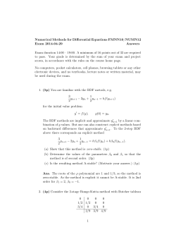
18
Figure 3.1: (a) A hydrogel scaffold (blue) containing dissolved growth factors (orange) is seeded
with sparsely distributed chondrocytes (red). (b) Over time, the chondrocytes synthesize new
ECM (white). (c) In this chapter, the model describes interactions in the local environment of
a single chondrocyte where cell-synthesized unlinked ECM (green) is transformed into linked
ECM (white) using growth factors (orange).
3.2
Primary Variables
The primary variables in this system are now summarized. Biomechanical variables, include
the solid phase displacement (us ), fluid phase velocity (vω ), pore pressure (p) of the interstitial
fluid and the water volume fraction or porosity (φω ). The evolution of bound constituents is
tracked by volume fractions φβ where the constituents β are chosen to be linked ECM (LM )
and scaffold (Sc). Similarly the unbound constituents can be represented by volume fractions
φα where the constituents α are chosen to be unlinked ECM (U M ) and growth-factor (G).
However, the unbound constituents are dissolved in the interstitial fluid and assumed to occupy
negligible mixture volume. Hence, in the model formulation, their evolution is tracked using
both concentrations (cU M ) and (cG ) and velocities (v U M ) and (v G ). Based on the choice of
these primary variables and the relations
ρβ = φβ ρβT , (β = ω, LM, Sc), and ρα = φω cα Mα , (α = U M, G),
(3.1)
the spatio-temporal PDE model that was presented in section 2.3 can be written as:
Mass Balance
∂t φω + ∇ · (vω φω ) = 0,
(3.2)
∂t φLM + ∇ · (u˙ s φLM ) = F LM (φω , φLM , φSc , cU M , cG ),
(3.3)
19
∂t φSc + ∇ · (u˙ s φSc ) = F Sc (φω , φLM , φSc , cU M , cG ),
∂t φω cU M + ∇ · (vU M φω cU M ) = F U M (φω , φLM , φSc , cU M , cG ),
∂t φω cG + ∇ · (vG φω cG ) = F G (φω , φLM , φSc , cU M , cG ).
(3.4)
(3.5)
(3.6)
Saturated Mixture
φs + φω = 1,
where : φs = φLM + φSc ,
φU M ≈ 0 φG ≈ 0,
(3.7)
Momentum Balance
−∇p + ∇ · σ E (us ) = 0,
(3.8)
−ρωT φω ∇µω (p, cU M , cG ) + f ωs (u˙ s − vω ) + f ω(U M ) (vU M − vω ) + f ωG (vG − vω ) = 0,
(3.9)
−MU M φω cU M ∇µU M (cU M ) + f s(U M ) (u˙ s − vU M ) + f ω(U M ) (vω − vU M ) = 0,
(3.10)
−MG φω cG ∇µG (cG ) + f sG (u˙ s − vG ) + f ωG (vω − vG ) = 0,
(3.11)
Constitutive Equations
σ E (us ) = λtr(es )I + 2µes , where: es = 1/2 (∇us ) + (∇us )t
µω (p, cU M , cG ) =
p
− φ(cU M + cG ),
RT
(3.12)
(3.13)
µU M (cU M ) = γU M cU M ,
(3.14)
µG (cG ) = γG cG .
(3.15)
The equations as formulated above are now specialized to the case of a one-dimensional spherical
model.
3.3
One Dimensional Spherical Model of a Cell Seeded in a
Porous Scaffold
In this model two regions are considered (Figure 3.2), an inner spherical region (Region 1)
that represents a cell with radius a and an outer spherical ring (Region 2) of dimension b that
represents the evolving extracellular region. The extracellular region is initially assumed to
contain only scaffold with interstitial fluid and dissolved growth factors while the cell is assumed
to contain a solid phase, interstitial fluid and dissolved solutes. Both regions are modeled as
saturated continuum mixtures.
A spherically symmetric model is developed by assuming that the kinematic variables. i.e.
20
Figure 3.2: Illustration of the initial configuration for one dimensional spherical model of a
single cell seeded in a scaffold.
solid displacements and fluid and solute velocities, are exclusively radial and depend on only
the radial coordinate (r) and time (t). Hence, in a spherical coordinate system
us = (us (t, r), 0, 0), vα = (v α (t, r), 0, 0), (α = w, U M, G),
3.3.1
(3.16)
Cell Region
The interaction function F α in section 2.3, equation (2.21), where α = U M is chosen to be
F
UM
ω
s
UM
(ρ , ρ , ρ
ρU M
UM
φω .
) = kU M N ρ∗ − ω
φ
∗
(3.17)
By using (3.1) and the following relation involving the critical unlinked ECM density within
the surrounding interstitial fluid
M
M
ρU
= cU
∗
∗ MU M ,
(3.18)
M
− cU M φω .
F U M (φω , φs , cU M ) = kU M N ∗ cU
∗
(3.19)
we obtain
Also, the constitutive law for the solid phase elastic stress σ E in (3.8) is written as:
σ E (us ) = λc tr(es )I + 2µc es
(3.20)
where (λc , µc ) are the elastic Lam´e coefficients for the cell. Governing equations for the cell
region are formulated for 0 < r < a and t > 0 as follows:
21
Mass Balance:
∂t φω +
s
∂t φ +
ω UM
∂t (φ c
)+
∂
2
+
∂r r
∂
2
+
∂r r
∂
2
+
∂r r
(v ω φω ) = 0,
(3.21)
(u˙ s φs ) = 0,
(3.22)
M
(v U M φω cU M ) = kU M N ∗ (cU
− cU M )φω .
∗
(3.23)
Saturated Mixture:
φs + φω = 1,
Momentum Balance:
∂p
∂
−
+ (λc + 2µc )
∂r
∂r
−ρωT φω
−MU M φω cU M
φU M ≈ 0,
∂us 2 s
+ u
∂r
r
(3.24)
= 0,
(3.25)
∂ ω
µ + f ωs (u˙ s − v ω ) + f ω(U M ) (v U M − v ω ) = 0,
∂r
(3.26)
∂ UM
µ
+ f s(U M ) (u˙ s − v U M ) + f ω(U M ) (v ω − v U M ) = 0.
∂r
(3.27)
In (3.23), kU M [(s·mol/L)−1 ] is the unlinked ECM synthesis rate and N ∗ [(mol/L)] is a saturated
nutrient concentration, based on the assumption that diffusive transport of small solutes is fast
relative to transport mechanisms of synthesized ECM constituents. Production of unlinked ECM
is assumed to proceed until the critical unlinked ECM concentration within the surrounding
M is reached within the surrounding interstitial fluid.
interstitial fluid cU
∗
3.3.2
Extracellular Region
The interaction functions F β and F α in section 2.3 where β = LM, Sc and α = U M, G are
chosen to be
F LM (ρω , ρLM , ρSc , ρU M , ρG ) = f (φs )ρU M ρG ,
(3.28)
F Sc (ρω , ρLM , ρSc , ρU M , ρG ) = −kSc ρSc ,
(3.29)
F U M (ρω , ρLM , ρSc , ρU M , ρG ) = −f (φs )ρU M ρG ,
(3.30)
F G (ρω , ρLM , ρSc , ρU M , ρG ) = −f (φs )ρU M ρG ,
(3.31)
Using the relations in (3.1), these functions can be represented in terms of our primary variables
as:
F LM (φω , φLM , φSc , cU M , cG ) =
f (φs )MU M MG ω 2 U M G
(φ ) c c ,
ρLM
T
F Sc (φω , φLM , φSc , cU M , cG ) = −kSc φSc ,
22
(3.32)
(3.33)
F U M (φω , φLM , φSc , cU M , cG ) = −f (φs )MG (φω )2 cU M cG ,
(3.34)
F G (φω , φLM , φSc , cU M , cG ) = −f (φs )MU M (φω )2 cU M cG .
(3.35)
Also, the solid phase elastic stress in the extracellular region (scaffold region) is defined by
σ E (us ) = λSc tr(es )I + 2µSc es ,
(3.36)
where (λSc , µSc ) are the elastic Lam´e coefficients in the scaffold region and this relation for σ E
is used in (3.8). Governing equations for the extracellular region are formulated for a < r < b
and t > 0 as follows:
Mass Balance:
ω
∂t φ +
∂t φ
LM
+
∂
2
+
∂r r
∂
2
+
∂r r
(u˙ s φLM ) =
(v ω φω ) = 0,
(3.37)
f (φs )MU M MG ω 2 U M G
(φ ) c c ,
ρLM
T
2
∂
+
(u˙ s φSc ) = −kSc φSc ,
∂t φ +
∂r r
∂
2
ω UM
∂t (φ c ) +
+
(v U M φω cU M ) = −f (φs )MG (φω )2 cU M cG ,
∂r r
Sc
(3.38)
∂t (φω cG ) + ∇ · (vG φω cG ) = −f (φs )MU M (φω )2 cU M cG ,
(3.39)
(3.40)
(3.41)
Saturated Mixture:
φs + φω = 1,
Momentum Balance:
−ρωT φω
where : φs = φLM + φSc ,
∂
∂p
+ (λSc + 2µSc )
−
∂r
∂r
φUM ≈ 0, , φG ≈ 0,
∂us 2 s
+ u
∂r
r
= 0,
∂ ω
µ + f ωs (u˙ s − v ω ) + f ω(U M ) (v U M − v ω ) + f ωG (v G − v ω ) = 0,
∂r
−MU M φω cU M
∂ UM
µ
+ f s(U M ) (u˙ s − v U M ) + f ω(U M ) (v ω − v U M ) = 0,
∂r
−MG φω cG
(3.42)
∂ G
µ + f sG (u˙ s − v G ) + f ωG (v ω − v G ) = 0.
∂r
(3.43)
(3.44)
(3.45)
(3.46)
The linking rate f (φs ) that appears in (3.38), (3.40), and (3.41) is modeled using as a
Gaussian distribution with respect to the solid phase volume fraction φs , similar to the ODE
23
model in Section 2.2 as:
(φs − φs∗ )2
,
f (φ ) = kU L exp −
2σ 2
s
(3.47)
where kU L [(s · kg/L)−1 ] is the maximum linking rate, occurring when φs = φs∗ . In (3.47), the
parameters φs∗ and σ define regimes in which rates for formation of linked ECM are enhanced
or inhibited. At low solid volume fraction φs , linking is assumed to increase with increasing φs
due to cell-scaffold biocompatibility. However, as φs increases past φs∗ , the linking rate begins
to slow down with decreasing average porosity φω = 1 − φs , to capture adverse effects on the
ability of unlinked ECM to form linked ECM as the pore size in the evolving tissue construct
reduces.
The term on the right hand side of (3.38) represents the interaction between the synthesized
unlinked ECM and the growth factor that facilitates assembly of the unlinked ECM into linked
ECM. Specifically, ECM linking is assumed to be regulated by both product inhibition and a
continuous set of linking rates f [(s · kg/L)−1 ] that depend on the time-varying average solid
volume fraction φs in the construct, as modeled in (3.47).
In (3.39), kSc [s−1 ] is the scaffold degradation rate. Terms on the right hand side of (3.40)
and (3.41) describe how unlinked ECM and growth factors are utilized in the system to produce
linked ECM.
3.3.3
Initial, Boundary and Interface Conditions
To complete the model formulation we must specify initial conditions on the two-zone spherical
domain (0 < r < b), boundary conditions at r = 0, b, and interface conditions along the fixed
interface, which corresponds to the cell membrane, at r = a. Initially, in a cartilage cell-scaffold
system, the cell is seeded within a scaffold of known initial porosity that is assumed to have a
uniform concentration of growth factor. Initially, it is also assumed that the system is at rest
and free of any unlinked or linked ECM. The resulting initial conditions for 0 < r < b are:
p(0, r) = 0,
cG (0, r) = cG
0,
φSc (0, r) = φSc
0 ,
φLM (0, r) = 0,
cU M (0, r) = 0,
(3.48)
us (0, r) = 0.
(3.49)
On the cell boundary r = a, interface conditions consist of continuity relations for the solid
phase normal stress and the water and unlinked ECM fluxes relative to the solid phase:
E
E
σrr
= σrr
,
r=a−
r=a+
(3.50)
φω (v ω − u˙ s )|r=a− = φω (v ω − u˙ s )|r=a+ ,
(3.51)
24
φω cU M (v U M − u˙ s )r=a− = φω cU M (v U M − u˙ s )r=a+ ,
(3.52)
The cell membrane is assumed to be impermeable to scaffold (Sc), linked ECM (LM ), and
growth factor (G) present in the extracellular region, leading to the no-flux conditions
∂φSc
(t, a+ ) = 0,
∂r
∂φLM
(t, a+ ) = 0,
∂r
∂cG
(t, a+ ) = 0.
∂r
(3.53)
Based on symmetry and physical constraints, boundary conditions at the center of the cell are
∂cU M
(t, 0) = 0,
∂r
∂φω
(t, 0) = 0,
∂r
us (t, 0) = 0,
∂p
(t, 0) = 0.
∂r
(3.54)
The outer boundary of the extracellular region (r = b) is assumed to lie in the far-field region
of the system. This boundary is assumed to be stress-free and no-flux conditions are prescribed
for the scaffold, linked matrix, unlinked matrix, and growth factor leading to the boundary
conditions
E
σrr
(t, b) = 0,
p(t, b) = 0,
∂φSc
(t, b) = 0,
∂r
∂φLM
(t, b) = 0,
∂r
∂cU M
(t, b) = 0,
∂r
(3.55)
∂cG
(t, b) = 0,
∂r
(3.56)
The resulting one-dimensional spatio-temporal cartilage regeneration model then consists of the
equations (3.21)-(3.27) and equations (3.37)-(3.46) subject to the conditions (3.48)-(3.56).
3.4
Model Reduction
The model developed in the previous section can be further reduced. Adding together (3.21)
and (3.22) and using the fact the mixture is saturated (3.42), we obtain the reduced equation
∂ 2 ω ω
(r (φ v + (1 − φω )u˙ s )) = 0.
∂r
(3.57)
Integrating with respect to r gives
(φω v ω + (1 − φω )u˙ s ) = f (t)/r2 ,
(3.58)
where f (t) is an arbitrary function. Since our solutions must be bounded for all time at r = 0,
we take f (t) = 0, giving the relation
φω v ω + (1 − φω )u˙ s = 0
25
(3.59)
which will be used in the place of (3.22). Again, using the fact that the mixture is saturated
(3.42) and the approximations φU M ≈ 0 and φG ≈ 0, (3.37) is replaced by the summation of
(3.37)-(3.39), leading to the reduced equation:
∂
2
+
∂r r
(v ω φω + u˙ s (1 − φω )) = −kSc φSc +
f (φs )MU M MG ω 2 U M G
(φ ) c c
ρLM
T
(3.60)
The diffusive drag coefficients between phases in our mixture can be related to solute diffusivities using the relations [64]
f ωs =
φω
,
k
f ω(U M ) =
RT φω cU M
,
Dω(U M )
f ωG =
RT φω cG
.
DωG
(3.61)
In (3.61), k is the hydraulic permeability constant, Dω(U M ) , and DωG are the diffusivities of
unlinked ECM and growth factor, respectively, in water. Dω(U M ) , and DωG are assumed to be
functions of φω as defined in [17] by
Dω(U M ) =
DU M (φω )2
,
(2 − φω )2
DωG =
DG (φω )2
,
(2 − φω )2
(3.62)
where DU M and DG are the diffusivity of unlinked matrix ECM and the growth factor, respectively, in free solution. Similar to the approach used in [64], we assume that f s(U M ) ≈ 0 and
f sG ≈ 0.
Based on the transformed relations above, the full 1D model is now re-written in a simpler
form. In doing so, we substitute µω from (3.13) in (3.26) and (3.44), µU M from (3.14) in (3.27)
and (3.45), and µG from (3.15) in (3.46). Also, substituting the diffusive drag coefficients (3.61)
in (3.26), (3.27), (3.44), (3.45), and (3.46), the equations (3.26), (3.27), (3.44), (3.45), and (3.46)
become linear equations in v ω , v U M , and v G . We solve the linear system (3.26) and (3.27) for
v ω , v U M and the linear system (3.44), (3.45), and (3.46) for v ω , v U M , and v G . Lastly, we
substitute the relations obtained for v ω , v U M , and v G into all relevant equations to eliminate
these variables. The reduced model is now summarized for each region in the following two
subsections.
3.4.1
Cell Region
In the cell region, the reduced model contains four dependent variables that are the pore
pressure (p), solid phase displacement (us ), water volume fraction (φω ), and unlinked ECM
concentration (cU M ). For 0 < r < a and t > 0, the reduced governing equations are:
∂
∂p
−
+ (λc + 2µc )
∂r
∂r
26
∂us 2 s
+ u
∂r
r
= 0,
(3.63)
∂t φω +
u˙ s = k
ω UM
∂t (φ c
)+
∂
2
+
∂r r
∂
2
+
∂r r
[(φω − 1) u˙ s ] = 0,
∂p
∂cU M
− RT k(φ − 1)
,
∂r
∂r
(3.64)
(3.65)
UM
ω
UM s
ω(U M ) ω ∂c
(φ − 1)c u˙ − D
φ
=
∂r
M
kU M N ∗ (cU
− cU M )φω . (3.66)
∗
3.4.2
Extracellular Region
In the extracellular region, the reduced model contains six dependent variables that are the
pore pressure (p), solid phase displacement (us ), linked ECM, and scaffold volume fractions
(φLM and φSc ), and unlinked ECM and growth factor concentrations (cU M and cG ). We note
that the porosity φω can be determined from φLM and φSc since the mixture is saturated. For
a < r < b and t > 0, the reduced governing equations are:
∂p
∂
−
+ (λSc + 2µSc )
∂r
∂r
∂
2
+
∂r r
∂us 2 s
+ u
∂r
r
= 0,
(3.67)
UM
∂p
∂c
∂cG
s
−k
+ RT k(φ − 1)
+
+ u˙ =
∂r
∂r
∂r
f (φs )MU M MG ω 2 G U M
− kSc φSc +
(φ ) c c , (3.68)
ρLM
T
∂t φ
LM
+
2
∂
+
∂r r
∂t φ
ω UM
∂t (φ c
)+
Sc
(u˙ s φLM ) =
+
∂
2
+
∂r r
f (φs )MU M MG ω 2 G U M
(φ ) c c ,
ρLM
T
(u˙ s φSc ) = −kSc φSc ,
(3.69)
(3.70)
UM
U M ∂p
UM
ω(U M ) ω ∂c
ω UM s
−kc
+ RT k(φ − 1)c
−D
φ
+ φ c u˙
∂r
∂r
G
∂
2
U M ∂c
+
+
RT k(φ − 1)c
= −f (φs )MG (φω )2 cG cU M , (3.71)
∂r r
∂r
∂
2
+
∂r r
27
ω G
∂t (φ c ) +
3.4.3
∂
2
+
∂r r
G
G ∂p
G
ωG ω ∂c
ω G s
−kc
+ RT k(φ − 1)c − D φ
+ φ c u˙
∂r
∂r
∂cU M
∂
2
RT k(φ − 1)cG
= −f (φs )MG (φω )2 cG cU M . (3.72)
+
+
∂r r
∂r
Initial, Boundary, and Interface Conditions
For the four variables that are present in both the cell and extracellular regions, we have the
initial conditions for 0 < r < b:
(
cU M (0, r) = 0,
p(0, r) = 0,
us (0, r) = 0,
φω (0, r) =
(φω0 )c
0<r<a
(φω0 )Sc
a<r<b
. (3.73)
In the extracellular region (a < r < b), initial conditions for the additional variables are:
cG (0, r) = cG
0,
φLM (0, r) = 0,
(3.74)
where we note that the initial solid phase volume fraction in the extracellular region is φs0 =
1 − (φω0 )Sc .
At the cell center (r = 0), the boundary conditions are
∂cU M
(t, 0) = 0,
∂r
∂φω
(t, 0) = 0,
∂r
us (t, 0) = 0,
∂p
(t, 0) = 0,
∂r
(3.75)
and at the interface (r = a) between the cell and the extracellular region, the interface conditions
become:
(λc + 2µc )
∂us
∂r
s
2λc s ∂u
2λSc s +
u = (λSc + 2µSc )
+
u ,
r
∂r
r
r=a−
r=a+
∂p
∂cU M ∂cU M ∂p
−k
+ RT k(φ − 1)
= −k
+ RT k(φ − 1)
,
∂r
∂r r=a−
∂r
∂r r=a+
−kc
UM
(3.76)
(3.77)
UM ∂p
UM
U M ω ∂c
+ RT k(φ − 1)c
−D φ
=
∂r
∂r r=a−
UM
−kc
∂φSc
(t, a) = 0,
∂r
UM ∂p
UM
U M ω ∂c
+ RT k(φ − 1)c
−D φ
, (3.78)
∂r
∂r r=a+
∂φLM
(t, a) = 0
∂r
,
∂cG
(t, a) = 0.
∂r
(3.79)
Finally, at the outer boundary of the extracellular region (r = b), the boundary conditions
28
become:
(λSc + 2µSc )
p(t, b) = 0,
∂φSc
(t, b) = 0,
∂r
∂us
∂r
2λSc s +
u = 0,
r
r=b
∂φLM
(t, b) = 0,
∂r
∂cU M
(t, b) = 0,
∂r
(3.80)
∂cG
(t, b) = 0.
∂r
(3.81)
The system of equations above consists of the simplified equations (3.63)-(3.66) and (3.67)(3.72) subject to the conditions (3.74)-(3.81). Prior to considering finite difference schemes for
the numerical solution of this system, the system of equations is nondimensionalized, as outlined
in the next section.
3.5
Nondimensionalization
The system is nondimensionalized to facilitate a parametric analysis of interactions among
mechanisms captured in the model and to prevent ill conditioning of the linear algebraic system associated with the discretized governing equations. The following transformations are
introduced and all nondimensional variables are indicated using the hat notation ˆ·
rˆ =
r ˆ D0
cU M
a s
cG
us ˆs
p
, t = 2 t, cˆU M =
˙ =
, cˆG =
, u
ˆs = , u
u˙ , pˆ = α .
a
a
c0
c0
a
D0
HA
(3.82)
In the equations above, a, c0 , and D0 are characteristic scales for the cell radius, concentration,
and diffusivity, respectively and
α
HA
= λα + 2µα ,
(3.83)
where α represent the cell (c) and the scaffold (Sc). Substituting (3.82) into (3.63)-(3.81) yields
the following nondimensionalized model
3.5.1
Cell Region
For 0 < rˆ < 1 and tˆ > 0, the nondimensionalized governing equations are:
ˆs 2 ∂ u
ˆs
2 s
∂ pˆ ∂ 2 u
+
+
− 2u
ˆ = 0,
∂ rˆ
∂ rˆ2
rˆ ∂ rˆ
rˆ
i
∂
2 h ω
ω
ˆ˙s = 0,
+
(φ − 1) u
∂tˆφ +
∂ rˆ rˆ
−
(3.84)
(3.85)
UM
c
ˆ˙s = Rgc ∂ pˆ − Kg (φ − 1) ∂ˆ
u
,
∂ rˆ
∂ rˆ
29
(3.86)
ω UM
∂tˆ(φ cˆ
3.5.2
)+
∂
2
+
∂ rˆ rˆ
cU M
ω
U M ˆs
U M ω ∂ˆ
(φ − 1)ˆ
c u˙ − Dr φ
=
∂ rˆ
M
kˆU M N ∗ (ˆ
cU
− cˆU M )φω . (3.87)
∗
Extracellular Region
For 1 < rˆ < ˆb and tˆ > 0, the nondimensionalized governing equations are:
∂ pˆ ∂ 2 u
ˆs 2 ∂ u
ˆs
2 s
+
+
− 2u
ˆ = 0,
(3.88)
2
∂ rˆ
∂ rˆ
rˆ ∂ rˆ
rˆ
UM
ˆ
∂
2
∂ˆ
c
∂ˆ
cG
Sc ∂ p
s
ˆ
−Rg
+ u˙ = −kˆSc φSc + kˆ1 (φω )2 cˆG cˆU M ,
+
+ Kg (φ − 1)
+
∂ rˆ rˆ
∂ rˆ
∂ rˆ
∂ rˆ
(3.89)
∂
2
ˆ˙s φLM ) = kˆ1 (φω )2 cˆG cˆU M ,
∂tˆφLM +
+
(u
(3.90)
∂ rˆ rˆ
2 ˆs Sc
∂
+
(u˙ φ ) = −kˆSc φSc ,
(3.91)
∂tˆφSc +
∂ rˆ rˆ
−
ω UM
∂tˆ(φ cˆ
ω G
)+
∂tˆ(φ cˆ ) +
∂
2
+
∂ rˆ rˆ
2
∂
+
∂ rˆ rˆ
cU M
ˆ
Sc U M ∂ p
UM
U M ω ∂ˆ
ω U M ˆs
−Rg cˆ
+ Kg (φ − 1)ˆ
c
− Dr φ
+ φ cˆ u˙
∂ rˆ
∂ rˆ
∂
2
∂ˆ
cG
+
+
Kg (φ − 1)ˆ
cU M
= −kˆ2 (φω )2 cˆG cˆU M , (3.92)
∂ rˆ rˆ
∂ rˆ
cG
ˆ
Sc G ∂ p
G
G ω ∂ˆ
ω G ˆs
−Rg cˆ
+ Kg (φ − 1)ˆ
c − Dr φ
+ φ cˆ u˙
∂ rˆ
∂ rˆ
2
cU M
∂
G ∂ˆ
+
Kg (φ − 1)ˆ
c
= −kˆ3 (φω )2 cˆG cˆU M , (3.93)
+
∂ rˆ rˆ
∂ rˆ
where
Rgc =
DrG =
c
Sc
kHA
kHA
RT kc0
, RgSc =
, Kg =
,
D0
D0
D0
DωG
Dω(U M ) ˆ
a2
a2
, DrU M =
, kU M =
kU M , kˆSc =
kSc ,
D0
D0
D0
D0
f (φs )(MU M )2 c20 a2 ˆ
c0 a2 ˆ
c0 a2
s
s
kˆ1 =
,
k
=
f
(φ
)M
,
k
=
f
(φ
)M
.
2
3
G
U
M
D0
D0
D0
ρLM
T
30
(3.94)
(3.95)
(3.96)
3.5.3
Initial, Boundary, and Interface Conditions
For both the cell and extracellular regions, we have the nondimensionalized initial conditions
for 0 < rˆ < ˆb:
(
cˆU M (0, rˆ) = 0,
pˆ(0, rˆ) = 0,
u
ˆs (0, rˆ) = 0,
φω (0, rˆ) =
(φω0 )c
(φω0 )Sc
0 < rˆ < 1
1 < rˆ < ˆb.
(3.97)
In the extracellular region (1 < rˆ < ˆb), initial conditions for the additional variables are:
cˆG (0, rˆ) =
cG
0
,
c0
φLM (0, rˆ) = 0,
(3.98)
where φs0 = 1 − (φω0 )Sc in the extracellular region.
At the center of the cell (ˆ
r = 0), the nondimensionalized boundary conditions are
∂ˆ
cU M ˆ
(t, 0) = 0,
∂ rˆ
∂φω ˆ
(t, 0) = 0,
∂ rˆ
∂ pˆ ˆ
(t, 0) = 0,
∂ rˆ
u
ˆs (tˆ, 0) = 0,
(3.99)
and at the interface (ˆ
r = 1) between the cell and the extracellular region, the nondimensionalized
interface conditions become:
s
s
∂u
ˆ
2λc s ∂u
ˆ
2λSc s (λc + 2µc )
+
u
ˆ = (λSc + 2µSc )
+
u
ˆ ,
∂ rˆ
rˆ
∂ rˆ
rˆ
rˆ=1−
rˆ=1+
∂ˆ
cU M ˆ
∂ˆ
cU M Sc ∂ p
+ RT c0 (φ − 1)
= −HA
+ RT c0 (φ − 1)
,
∂ rˆ
∂ rˆ r=1−
∂ rˆ
∂ rˆ r=1+
ˆ
c ∂p
−HA
c UM
−HA
cˆ
∂ pˆ
+
∂ rˆ
UM
RT c0 (φ − 1)ˆ
c
Dω(U M ) ω
−
φ
k
!
∂ˆ
cU M ∂ rˆ ˆ
Sc U M ∂ p
−HA
cˆ
+
∂ rˆ
RT c0 (φ − 1)ˆ
cU M −
∂φSc ˆ
(t, 1) = 0,
∂ rˆ
∂φLM ˆ
(t, 1) = 0,
∂ rˆ
(3.100)
(3.101)
=
rˆ=1−
Dω(U M )
k
!
φω
∂ˆ
cG ˆ
(t, 1) = 0.
∂ rˆ
∂ˆ
cU M ∂ rˆ , (3.102)
rˆ=1+
(3.103)
At the outer boundary of the extracellular region (ˆ
r = ˆb), the nondimensionalized boundary
conditions become:
(λSc + 2µSc )
∂u
ˆs
∂ rˆ
31
2λ s +
u
ˆ
= 0,
rˆ rˆ=ˆb
(3.104)
pˆ(tˆ, ˆb) = 0,
∂φSc ˆ ˆ
(t, b) = 0,
∂ rˆ
∂φLM ˆ ˆ
(t, b) = 0,
∂ rˆ
32
∂ˆ
cU M ˆ ˆ
(t, b) = 0,
∂ rˆ
∂ˆ
cG ˆ ˆ
(t, b) = 0. (3.105)
∂ rˆ
Chapter 4
Numerical Methods and Simplified
Analytical Solution for Verification
4.1
Introduction
The finite difference method is used to formulate a numerical scheme for the approximate
solution of the nondimensionalized system (3.84)-(3.93) subject to the boundary and interface
conditions (3.97)-(3.105). The application of the resulting numerical scheme to the simulation of
cartilage ECM regeneration results is discussed in Chapter 5. The spatio-temporal PDE model
developed in the previous chapter is formulated in two regions and is comprised of several
PDEs formulated in terms of multiple unknowns, along with both boundary and interface
conditions. Furthermore, numerical stability conditions for this system of governing equations
are unknown. For these reasons, an analytical solution for verification of the numerical scheme
is also developed in this chapter and used to evaluate accuracy of both the scheme and its
implementation in MATLAB.
4.2
Numerical Scheme
We discretize the spatial and temporal domains using fixed step sizes ∆ˆ
r and ∆tˆ, respectively.
In the cell region, the non-dimensional spatial step size is taken as ∆ˆ
r = 1/m, where m is
prescribed. In the extracellular region, the same spatial step size ∆ˆ
r is used and the location
of the outer boundary b is adjusted to align with the mesh. The temporal step size is taken to
be ∆tˆ = tˆf /n, where the final time in the simulation tf is prescribed.
To approximate the numerical solutions at every time step of the nondimensionalized equations in the cell region (3.84)-(3.87), let pˆji = pˆ(tˆj , rˆi ), (ˆ
us )ji = u
ˆs (tˆj , rˆi ), (φω )ji = φω (tˆj , rˆi ),
(ˆ
cU M )ji = cˆU M (tˆj , rˆi ) for i = 1, 2, ..., m − 1, j = 1, 2, ..., n, where rˆi = i∆ˆ
r, and tˆj = j∆tˆ. Note
33
that the numerical solution at the current time is at tˆ = tˆj+1 . The discretization of Equation
(3.84), which does not explicitly depend on time, is written as
−
us )j+1
∂ pˆj+1 ∂ 2 (ˆ
us )j+1 2 ∂(ˆ
2 s j+1
+
u )
= 0.
+
− 2 (ˆ
2
∂ rˆ
∂ rˆ
rˆ ∂ rˆ
rˆ
(4.1)
For (3.86) the time discretization is handled using backward Euler (implicit) time stepping so
that
(ˆ
us )j+1 − (ˆ
us )j
∂ pˆj+1
∂(ˆ
cU M )j+1
= Rgc
− Kg (φ − 1)
.
∂ rˆ
∂ rˆ
∆tˆ
(4.2)
The remaining two governing equations in the cell region (3.85) and (3.87) also depend explicitly
on time, but are nonlinear. The nonlinearity in equation (3.85) arises from a product of the
evolving porosity and the solid phase velocity. This equation is discretized to yield a linear
equation by using a backward Euler scheme for the solid phase velocity and treating the porosity
as an explicit term, i.e. evaluated at the previous time step:
(φω )j+1 − (φω )j
+
∆tˆ
∂
2
+
∂ rˆ rˆ
(ˆ
us )j+1 − (ˆ
us )j
(φ ) − 1
∆tˆ
ω j
= 0.
(4.3)
Similarly, (3.87) has nonlinear terms involving products of evolving porosity, solid phase velocity
and unlinked ECM concentration. These terms are also discretized to yield a linear discretized
equation. Backward Euler is used for terms involving the solid phase velocity and the gradient
of the unlinked ECM concentration, and all porosities are treated explicitly, i.e. evaluated at
the previous time step, resulting in the discrete equation:
(φω )j (ˆ
cU M )j+1 − (φω )j (ˆ
cU M )j
ˆ
∆t ∂
2
us )j+1 − (ˆ
us )j
cU M )j+1
ω j
U M j (ˆ
U M j ω j ∂(ˆ
+
+
((φ ) − 1)(ˆ
c )
− (Dr ) (φ )
∂ rˆ rˆ
∂ rˆ
∆tˆ
∗
U
M
U
M
j+1
= kˆU M N (ˆ
c∗ − (ˆ
c ) )(φω )j . (4.4)
Similarly, the techniques used above for both time discretization and treatment of nonlinear
terms are applied to discretize the remaining equations (3.88) through (3.93) resulting in the
following numerical scheme scheme for j = 1, 2, ..., n at points outside of the cell, i.e. i =
m + 1, m + 2, ..., M (the spatial discretization scheme is addressed at the end of this section):
−
∂ pˆj+1 ∂ 2 (ˆ
us )j+1 2 ∂(ˆ
us )j+1
2 s j+1
+
+
− 2 (ˆ
u )
= 0,
2
∂ rˆ
∂ rˆ
rˆ ∂ rˆ
rˆ
34
(4.5)
∂
2
+
∂ rˆ rˆ
ˆj+1
(ˆ
us )j+1 − (ˆ
us )j
∂(ˆ
cU M )j+1 ∂(ˆ
cG )j+1
Sc ∂ p
−Rg
+
+ Kg (φ − 1)
+
∂ rˆ
∂ rˆ
∂ rˆ
∆tˆ
= −kˆSc (φSc )j+1 + kˆ1 ((φω )j )2 (ˆ
cG )j (ˆ
cU M )j+1 , (4.6)
(φLM )j+1 − (φLM )j
+
∆tˆ
∂
2
+
∂ rˆ rˆ
us )j+1 − (ˆ
us )j
LM j (ˆ
(φ )
∆tˆ
= kˆ1 ((φω )j )2 (ˆ
cG )j (ˆ
cU M )j+1 , (4.7)
(φSc )j+1 − (φSc )j
+
∆tˆ
2
∂
+
∂ rˆ rˆ
us )j+1 − (ˆ
us )j
Sc j (ˆ
(φ )
= −kˆSc (φSc )j+1 ,
∆tˆ
(4.8)
(φω )j (ˆ
cU M )j+1 − (φω )j (ˆ
cU M )j
∆tˆ cU M )j+1
∂
2
ˆj+1
Sc U M j ∂ p
UM j
UM
ω j ∂(ˆ
+
+
−Rg (ˆ
c )
+ Kg (φ − 1)(ˆ
c ) − Dr (φ )
∂ rˆ rˆ
∂ rˆ
∂ rˆ
s
j+1
s
j
G
j+1
2
u )
− (ˆ
u )
c )
∂
ω j U M j (ˆ
U M j ∂(ˆ
+
(φ ) (ˆ
c )
+ Kg (φ − 1)(ˆ
c )
+
∂ rˆ rˆ
∂ rˆ
∆tˆ
ω
j
2
G
j
= −kˆ2 ((φ ) ) (ˆ
c ) (ˆ
cU M )j+1 , (4.9)
(φω )j (ˆ
cG )j+1 − (φω )j (ˆ
cG )j
ˆ
∆t
cG )j+1
∂
2
ˆj+1
Sc G j ∂ p
G j
G ω j ∂(ˆ
+
+
−Rg (ˆ
c )
+ Kg (φ − 1)(ˆ
c ) − Dr (φ )
∂ rˆ rˆ
∂ rˆ
∂ rˆ
U
M
s
j+1
s
j
∂
∂(ˆ
c )j+1
2
(ˆ
u )
− (ˆ
u )
+
+ Kg (φ − 1)(ˆ
cG )j
+
(φω )j (ˆ
cG )j
∂ rˆ rˆ
∂ rˆ
∆tˆ
= −kˆ3 ((φω )j )2 (ˆ
cU M )j (ˆ
cG )j+1 . (4.10)
Time discretization of the boundary conditions at rˆ = 0 are handed as:
∂(ˆ
cU M )j+1 ˆ
∂(φω )j+1 ˆ
∂(ˆ
p)j+1 ˆ
(t, 0) = 0,
(t, 0) = 0, (ˆ
us )j+1 (tˆ, 0) = 0,
(t, 0) = 0,
∂ rˆ
∂ rˆ
∂ rˆ
(4.11)
and time discretization of the interface conditions at rˆ = 1 are:
(λc + 2µc )
∂(ˆ
us )j+1
∂ rˆ
2λc s j+1 +
(ˆ
u ) =
r
r=1−
(λSc + 2µSc )
35
∂(ˆ
us )j+1
∂ rˆ
2λSc s j+1 +
(ˆ
u ) , (4.12)
r
rˆ=1+
p)j+1
c ∂(ˆ
−HA
∂ rˆ
∂(ˆ
cU M )j+1 + RT c0 (φ − 1)
−=
∂ rˆ
rˆ=1
p)
Sc ∂(ˆ
−HA
j+1
∂ rˆ
p)j+1
c U M j ∂(ˆ
−HA
(ˆ
c )
+
∂ rˆ
Sc U M j
−HA
(c )
∂(ˆ
p)j+1
+
∂ rˆ
∂(ˆ
cU M )j+1 + RT c0 (φ − 1)
+ , (4.13)
∂ rˆ
rˆ=1
∂(ˆ
cU M )j+1 =
−
∂ rˆ
r
ˆ
=1
!
ω(U M ) )j
U M )j+1 (D
∂(ˆ
c
RT c0 (φ − 1)(ˆ
cU M )j −
(φω )j
, (4.14)
+
k
∂ rˆ
(Dω(U M ) )j ω j
RT c0 (φ − 1)(ˆ
cU M )j −
(φ )
k
!
rˆ=1
∂(φSc )j+1 ˆ
∂(φLM )j+1 ˆ
∂(ˆ
cG )j+1 ˆ
(t, 1) = 0,
(t, 1) = 0,
(t, 1) = 0.
∂ rˆ
∂ rˆ
∂ rˆ
(4.15)
At the outer boundary of the extracellular region (ˆ
r = ˆb), the discretized boundary conditions become:
(λSc + 2µSc )
∂(ˆ
us )j+1
∂ rˆ
2λSc s j+1 = 0,
+
(ˆ
u ) rˆ
rˆ=ˆb
(4.16)
∂(φSc )j+1 ˆ ˆ
∂(φLM )j+1 ˆ ˆ
(ˆ
p)j+1 (tˆ, ˆb) = 0,
(t, b) = 0,
(t, b) = 0,
∂ rˆ
∂r
(4.17)
∂(ˆ
cU M )j+1 ˆ ˆ
∂(ˆ
cG )j+1 ˆ ˆ
(t, b) = 0,
(t, b) = 0.
∂ rˆ
∂r
(4.18)
It should be noted that, for simplicity of the presentation above, finite difference approximations for the spatial derivatives were not shown. All spatial derivatives above were discretized
using a second order difference (central differences) for the second order derivatives and a firstorder scheme for all first derivatives.
4.3
Simplified Model for Verification
In this section the full non-dimensional model is reduced to a simplified model that admits an
analytical solution. This analytical solution is applied to verify the accuracy and implementation
of the numerical scheme that was formulated in the previous section, with an emphasis on
temporal aspects of the problem.
For the cell region, both the solid displacement u
ˆs (tˆ, rˆ) and pore pressure pˆ(tˆ, rˆ) are assumed
to be zero. The unlinked matrix concentration is assumed to depend only on time, so that
∂ˆ
cU M /∂ rˆ = 0. Based on these assumptions, the equations (3.84) and (3.86) are automatically
satisfied. The remaining equations to be solved in the cell region are the reduced versions of
36
(3.85) and (3.87) which are
∂φω
= 0,
∂ tˆ
(4.19)
∂ˆ
cU M
M
= kˆU M N ∗ (ˆ
cU
− cˆU M ).
(4.20)
∗
ˆ
∂t
For the extra-cellular region, both solid displacement and pore pressure are assumed to be
zero, i.e. u
ˆs (tˆ, rˆ) = 0, and pˆ(tˆ, rˆ) = 0. It is also assumed that the growth factor concentration
(ˆ
cG ) is constant, and that the scaffold does not degrade, i.e. kSc = 0. Lastly, we assume that
linked matrix does not form from unlinked matrix by taking kU L = 0 and the osmotic coefficient
φ is taken to be 1. These assumptions lead to satisfaction of (3.88), (3.89), and (3.93) and the
remaining equations (3.90), (3.91), and (3.92) reduce to:
∂φLM
=0
∂ tˆ
∂φSc
=0
∂ tˆ
∂ˆ
cU M
∂
2
cU M
U M ∂ˆ
+
+
−Dr
=0
∂ rˆ rˆ
∂ rˆ
∂ tˆ
(4.21)
(4.22)
(4.23)
The initial conditions and boundary conditions at rˆ = 0 and rˆ = 1 are based on those for the
non-dimensionlized model in section 3.5. The interface conditions (3.100), (3.101), and (3.103)
are automatically satisfied, while the interface condition (3.102) mathematically reduces to:
∂ˆ
cU M = 0.
∂ rˆ rˆ=1+
(4.24)
However, since unlinked matrix concentration in the cell region is assumed to depend only
on time, the condition for flux continuity across the interface is replaced by a condition for
continuity of concentration that supplies cell-synthesized unlinked matrix to the extracellular
region via the modified interface condition:
cˆU M rˆ=1+ = cˆU M rˆ=1− .
(4.25)
Lastly, in the reduced model, the outer boundary of the extracellular region ˆb is chosen to
have the dimensionless value 2. The full set of governing equations for the reduced model is
summarized below.

ω
 ∂φ = 0
tˆ ≥ 0, 0 ≤ rˆ ≤ 1
∂ tˆ
 φω (0, rˆ) = (φω )c
0 ≤ rˆ ≤ 1
0
37
(4.26)












cU M ) ˆ
 ∂(ˆ
M
= kU M N ∗ (ˆ
cU
− cˆU M ) tˆ ≥ 0, 0 ≤ rˆ ≤ 1
∗
ˆ
∂
t
 UM
cˆ (0, rˆ) = 0
0 ≤ rˆ ≤ 1

LM
 ∂φ
=0
tˆ ≥ 0, 1 ≤ rˆ ≤ 2
ˆ
∂
t
 LM
φ (0, rˆ) = 0
1 ≤ rˆ ≤ 2

Sc
 ∂φ
=0
tˆ ≥ 0, 1 ≤ rˆ ≤ 2
ˆ
∂
t
 Sc
φ (0, rˆ) = φSc
1 ≤ rˆ ≤ 2
0
∂
cU M
∂ˆ
cU M
2
U M ∂ˆ
+
−Dr
= 0 tˆ ≥ 0, 1 ≤ rˆ ≤ 2
+
∂ rˆ rˆ
∂ rˆ
∂ tˆ
cˆU M (0, rˆ) = 0
1 ≤ rˆ ≤ 2
U
M
∂ˆ
c
(tˆ, 2) = 0
tˆ ≥ 0
cˆU M |rˆ=1+ = cˆU M |rˆ=1− ,
∂ rˆ
(4.27)
(4.28)
(4.29)
(4.30)
We observe that the reduced model effectively treats the cell region solution as a reaction,
i.e. variables are independent of rˆ, that interacts with a diffusion model for unlinked matrix
concentration in the extracellular region.
4.4
Analytical Solution of The Simplified Model
Equations (4.26), (4.27), (4.28), and (4.29) are ODEs that admit the following analytical solutions:
M
M −N ∗ kU M tˆ
φω (tˆ, rˆ) = 1 − φs0 , cˆU M (tˆ, rˆ) = cˆU
− cˆU
, φLM (tˆ, rˆ) = 0, φSc (tˆ, rˆ) = φSc
∗
∗ e
0 , (4.31)
respectively.
To find the analytical solution of (4.30) the method of separation of variables method was
used. For clarity of the presentation, the “hat” notation is dropped for the remainder of this
section.
Assume that
cU M (t, r) =
38
u(t, r)
r
(4.32)
Substituting (4.32) into (4.30) we obtain

2
∂u

UM ∂ u

=0
t ≥ 0, 1 ≤ r ≤ 2
−
D

r
 ∂t
∂r2
u(0, r) = 0
1≤r≤2



∂u
 u(t, 1) = cU M − cU M e−N ∗ kU M t , 2 (t, 2) − u(t, 2) = 0
t≥0
∗
∗
∂r
(4.33)
(4.33) is a diffusion equation with nonhomogeneous boundary conditions. It can be transformed
into a diffusion equation with homogeneous boundary conditions via the change of variable
M
M −N
u(t, r) = v(t, r) + (cU
− cU
∗
∗ e
∗k
UM t
)r.
(4.34)
Substituting (4.34) into (4.33) we obtain

2
∂v

UM ∂ v
M ∗
−N ∗ kU M t

−
D
= −(cU
)r t ≥ 0, 1 ≤ r ≤ 2

r
∗ N kU M e
2
 ∂t
∂r
v(0, r) = 0
1≤r≤2



∂v
 v(t, 1) = 0, 2 (t, 2) − v(t, 2) = 0
t≥0
∂r
(4.35)
Note that the PDE above is a nonhomogeneous diffusion equation but now has homogeneous
boundary conditions. The solution is assumed to be of the form v(t, r) = R(r)T (t). By ignoring
the source term in (4.35), we first find the eigenvalues and eigenfunctions of R(r) by solving
the problem
(
R00 + αR = 0
1≤r≤2
0
R(1) = 0, 2R (2) − R(2) = 0.
(4.36)
When α < 0, we write α = −λ2 and the equation for R becomes
R00 − λ2 R = 0,
which has general solution
R(r) = c1 cosh(λr) + c2 sinh(λr).
The condition R(1) = 0 gives
c1 = −
sinh(λ)
c2 .
cosh(λ)
The value of c1 resulting from enforcing the boundary condition 2R0 (2) − R(2) = 0 above gives
c2 [− sinh(λ)(2λ sinh(2λ) − cosh(2λ)) + cosh(λ)(2λ cosh(2λ) − sinh(2λ))] = 0.
39
If c2 6= 0, it can be readily shown (e.g. using MAPLE) that the term inside the bracket is never
zero for λ < 0. Thus, c2 = 0 and the case α < 0 yields only trivial solutions.
Similarly in the case α = 0, the differential equation reduces to R00 = 0 with general solution
R(r) = c1 r + c2 . The only way to satisfy the boundary conditions on R is to take c1 = c2 = 0
which again leads to the trivial solution R = 0. In the only remaining case we have
α = λ2 > 0.
The corresponding boundary value problem in R is
(
R00 + λ2 R = 0
R(1) = 0,
2R0 (2)
1≤r≤2
− R(2) = 0.
The general solution of the differential equation is
R(r) = c1 sin(λr) + c2 cos(λr).
The condition R(1) = 0 gives
c1 = −
cos(λ)
c2
sin(λ)
Substituting this expression for c1 into the second boundary condition 2R0 (2) − R(2) = 0 gives
c2 [− cos(λ)(2λ cos(2λ) − sin(2λ)) − sin(λ)(2λ sin(2λ) − cos(2λ))] = 0.
Assuming that c2 6= 0, we obtain the condition
− cos(λ)(2λ cos(2λ) − sin(2λ)) − sin(λ)(2λ sin(2λ) − cos(2λ)) = 0.
This equation has an infinite number of positive solutions λ1 , λ2 , ..... While we do not have
explicit formulas for the λn , approximate numerical values of the λn ’s can be determined using
MAPLE. Assuming that these eigenvalues can be computed, the solutions R(r) of (4.36) are
eigenfunctions that can be written as:
Rn (r) = sin(λn r) − tan(λn ) cos(λn r),
n = 1, 2, . . . ,
and the solution of (4.35) will be of the form
∞
X
v(t, r) =
(sin(λn r) − tan(λn ) cos(λn r))Tn (t).
n=1
40
(4.37)
Substituting (4.37) into (4.35) yields
∞
X
(sin(λn r) − tan(λn ) cos(λn r))Tn0 (t)−
n=1
DrU M
∞
X
M ∗
−N
(−λ2n sin(λn r) + λ2n tan(λn ) cos(λn r))Tn (t) = −(cU
∗ N kU M e
∗k
UM t
)r. (4.38)
n=1
Assuming that the right hand side of (4.35) has the same series form as v(t, r), we obtain
M ∗
−N ∗ kU M t
−(ˆ
cU
)r
∗ N kU M e
=
∞
X
(sin(λn r) − tan(λn ) cos(λn r))Fn (t).
(4.39)
n=1
This implies that
Fn (t) = Kn e−N
∗k
UM t
,
(4.40)
where Kn is a constant which can be written as
R2
Kn =
M ∗
−(cU
∗ N kU M )r(sin(λn r) − tan(λn ) cos(λn r))dr
1
R2
.
(sin(λn r) − tan(λn ) cos(λn
(4.41)
r))2 dr
1
Substituting (4.39) into (4.38) gives
(
Tn0 (t) + DrU M λ2n Tn (t) = Fn (t) t ≥ 0
Tn (0) = 0,
(4.42)
which is first a order ordinary differential equation. It can be solved for every positive integer
n ≥ 1 and the solution is
UM
Tn (t) =
2
∗
Kn (e−Dr λn t − e−N kU M t )
.
DrU M λ2n − N ∗ kU M
(4.43)
Then v(t, r), the solution of (4.35), can be written by substituting (4.43) into (4.37) to
obtain
UM 2
∗
∞
X
Kn (e−Dr λn t − e−N kU M t )
v(t, r) =
(sin(λn r) − tan(λn ) cos(λn r))
.
U M λ2 − N ∗ k
D
U
M
r
n
n=1
41
(4.44)
After finding the v(t, r) we can write u(t, r) as
M
M −N
u(t, r) = (cU
− cU
∗
∗ e
∗k
∞
X
UM t
)r+
UM
(sin(λn r) − tan(λn ) cos(λn r))
n=1
∗
2
Kn (e−Dr λn t − e−N kU M t )
. (4.45)
DrU M λ2n − N ∗ kU M
Lastly, the solution of (4.35) is thus obtained as:
M
M −N
cU M (t, r) = (cU
− cU
∗
∗ e
∞
X
∗k
UM t
)+
UM
(sin(λn r) − tan(λn ) cos(λn r))
n=1
4.5
2
∗
Kn (e−Dr λn t − e−N kU M t )
(DrU M λ2n − N ∗ kU M )r
(4.46)
Verification of Numerical Scheme Using The Simplified Model
(a)
(b)
Figure 4.1: Evaluation of the error between the numerical and simplified analytical solutions:
(a) Absolute value of the error as the mesh is refined based on the choices in Table 4.1 shown at
the time t=23.6 days, (b) a log-log plot of the infinity norm of the error between the numerical
and simplified analytical solutions at the time t=23.6 days demonstrating a first-order rate of
convergence.
We used the simplified model developed in the previous sections to verify accuracy and
implementation of the temporal aspects of the numerical method. The MATLAB code for
42
Table 4.1: Mesh sizes and infinity-norm error between the numerical and simplified analytical
solutions at the time t = 23.6 days.
m
50
100
200
300
400
500
600
700
800
color
Black
Red
Blue
Green
Yellow
Magenta
Cyan
Black
Red
||E||∞
0.0029
0.0016
8.6923x10−4
5.9061x10−4
4.4716x10−4
3.5976x10−4
3.0092x10−4
2.5863x10−4
2.2675x10−4
the full model, that was implemented based on the nondimensionlized model in Section 3.5,
was reduced to simulate the simplified model developed in this chapter. Note that the interface
conditions in the nondimensionlized model given by (3.100)-(3.103) were replaced by a simplified
boundary condition, as outlined in section 4.3, due to the fact the simplified model in the
cell region was independent of rˆ. All model parameters that appear in (4.27) and (4.30) were
assumed to have the same values that are used in the baseline case presented in the next chapter
(see Section 5.2 and Tables 5.1-5.3).
Let m and n to be the number of steps with respect to space (ˆ
r) and time (tˆ). For the
simplified model, the choice n = 6m yielded simulations that all exhibited numerical convergence as the mesh was refined. Let cˆU M and c˜ˆU M to be the analytic solution and the numerical
solution respectively. Define
E = cˆU M − c˜ˆU M and
||E||∞ = max cˆU M − c˜ˆU M .
0≤ˆ
r≤1
To illustrate numerical convergence rates of the method, E was found locally when tˆ = 2.5773x107
(i.e. t = 23.6 days) and is plotted versus rˆ with n = 6m in Figure 4.1a based on the mesh sizes
specified in Table 4.1 The numerical discretization in time, developed in section 4.1, exhibits
numerical convergence that is first order in time as seen in Figure 4.1b.
43
Chapter 5
Parametric Analysis and Results
5.1
Introduction
In this chapter, the spatio-temporal PDE continuum mixture model for cartilage extracellular
matrix regeneration in the local environment of a single cell is applied in a parametric analysis.
The investigation focuses on the effects of evolving scaffold porosity on accumulation of linked
ECM in the (extracellular) region surrounding the cell. The associated governing equations,
along with the interface and boundary conditions developed in Chapter 3, are solved using
the numerical discretization scheme outlined in Sec. 4.2. Results for evolution of the primary
variables in the model are illustrated in terms of a baseline set of parameter values. Several
of these values are fixed based on known physical or chemical properties of components of
the cell-scaffold system. Other parameter values that govern the physiological interactions of
system components are calibrated to yield ECM regeneration times that are on realistic scales
for tissue engineered articular cartilage. e.g. from a few weeks to several months.
5.2
Baseline Model Parameters
Parameters in the spatio-teporal PDE model described in Chapter 3 can be separated into three
main categories: biophysical parameters, scaffold design parameters, and physiological parameters. Although there is a fourth group which are geometric parameters, in a one-dimensional
model the primary geometric parameter is the cell radius whose value is well known for chondrocytes, e.g. a = 5x10−6 m is a typical radius of a chondrocyte [28]. In the non-dimensional
model (Sec. 3.5), this cell radius is used in setting rˆ = 1 as the location of the cell-scaffold interface. Based on this choice, the (far-field) outer boundary for the extracellular region is taken
as rˆ = 2. Also, there are several constants that have fixed values independent of interactions
within the cell-scaffold system. These are the universal gas constant (R = 8.31432 J/mol · K),
44
the absolute ambient temperature taken as T = 298 K and the osmotic coefficient (φ = 1) for
ideal solutions [41]. In addition, the nutrient concentration required to sustain biosynthesis in
living cells is fixed at a value of N ∗ = 0.1 mol/L [19]. Note that diffusion of these nutrients
was not modeled explicitly since these solutes are small relative to unlinked ECM and growth
factors and, as a result, their diffusion times are relatively fast.
5.2.1
Biophysical Parameters
In our model, biophysical parameters refer to parameters that govern passive material properties
of the system constituents and diffusive transport times. In referring to diffusivities of unbound
solutes, it is important to note the distinction between values in free solution versus those in
a porous mixture. Recall that the parameters DU M and DG denote the diffusivity of unlinked
ECM and the growth factor, respectively, in free solution. D0 is the reference diffusivity used to
nondimensionalize the other diffusivity parameters in (3.82) and was chosen to be the same as
DU M . In our system, we assume that the diffusivity of the growth factor (DG ) is significantly
less than the diffusivity of the unlinked ECM (DU M ) since diffusivity increases as particle size
decreases, and the molecular weight of unlinked ECM (MU M ) is assumed to be significantly less
than that of the growth factor (MG ). The choice D0 = DU M was made since unlinked ECM
is the smallest diffusing solute modeled in our system and, thus, the characteristic times for
slower phenomena such as diffusion of larger solutes, scaffold degradation and ECM linking will
occur on a larger time scale than O(1). Specific values for each of the diffusivities were chosen
based on values reported by Mauck et al. ([35],Table 1).
The elastic Lam´e coefficients of the solid phase (λ, µ) were related to the Young’s modulus (E) and the Poisson’s ratio (ν) in equation (2.29). For the cell, the values (Ec , νc ) =
c = λ + 2µ can also be
(1000 Pa, 0.35) were chosen. The value of the aggregate modulus HA
c
c
determined using equation (2.29) and (3.83). In the extracellular region, which is initially scaffold, the values (ESc , νSc ) = (10Ec , 0.1) were chosen. Lastly, the true density of linked matrix
3
(ρLM
T ) was fixed at a value of 1.3x10 kg/L [48]. The choice of all biophysical parameter values
in the baseline case is summarized in Table 5.1.
5.2.2
Scaffold Design Parameters
The scaffold design parameters include the initial scaffold solid volume fraction (φSc
0 ) as well as
the hydraulic permeability (k). The initial scaffold porosity was chosen to be 98% corresponding
to a value of φSc
0 = 0.02 [19]. In the parametric analysis conducted later in this chapter, the
effects of varying the value of φSc
0 on the spatial-temporal accumulation of linked ECM in the
region around the cell is considered. The hydraulic permeability constant was chosen to have
a value k = 51.4x10−15 m4 /N · s, based on [35] (Table 2). The scaffold design parameter values
45
Table 5.1: Biophysical parameter values that are used to analyze the spatio-temporal PDE
model in the baseline case.
Parameter
DU M
DG
D0
MU M
MG
(Ec , νc )
Description
Diffusivity of unlinked matrix in free solution
Diffusivity of the growth factor in free solution
Reference diffusivity
Molecular weight of unlinked matrix
Molecular weight of growth factor
Young’s modulus and Poisson’s ratio for the cell
λc
First elastic Lam´e coefficient for the cell
µc
Second elastic Lam´e coefficient (shear modulus)
for the cell
Young’s modulus and Poisson’s ratio for the
scaffold (extracellular region)
(ESc , νSc )
λSc
First elastic Lam´e coefficient for the scaffold
(extracellular region)
µSc
Second elastic Lam´e coefficient (shear modulus)
for the scaffold (extracellular region)
True density of linked matrix
ρLM
T
46
Value
3.16x10−10 (m2 /s)
6.97x10−11 (m2 /s)
DU M
20 (kg/mol)
67 (kg/mol)
(1000 Pa, 0.35)
Ec νc
(1 + νc )(1 − 2νc )
Ec
2(1 + νc )
Ref.
[17],[35]
[17],[35]
[35]
[35]
[35]
(10Ec , 0.1)
ESc νSc
(1 + νSc )(1 − 2νSc )
ESc
2(1 + νSc )
1.3x103 (kg/L)
[48]
Table 5.2: Parameter values for the scaffold that are used to analyze the spatio-temporal PDE
model in the baseline case.
Parameter
φSc
0
k
Description
Initial scaffold solid volume fraction
Hydraulic permeability
Value
0.02
−15
51.4x10
(m4 /N · s)
Ref.
[19]
[35]
for the baseline case are summarized in Table 5.2.
5.2.3
Physiological Parameters
We refer to physiological parameters in our model as those that govern phenomena regulated by
the biological cells in a tissue engineered construct. The first important parameter is the critical
M = cU M /c . This parameter is based on the phenomena of
unlinked matrix concentration cˆU
0
∗
∗
product inhibition in tissue engineered cartilage [8]. In this context, product inhibition refers
to the observation that the rate of cell-mediated biosynthesis of ECM components slows down
as the total amount produced increases. The specific formulation in our model is based on the
hypothesis that the cell detects the concentration of unlinked matrix in the fluid phase within
M was made by taking the critical unlinked matrix density (¯
M
the cell. The choice of cˆU
ρU
∗
∗ ) in
(3.18) and converting it to a concentration in moles of solute per volume of solvent, using the
molecular weight of unlinked matrix (MU M ), where the solvent is the fluid phase of the mixture.
Note that the characteristic unlinked matrix concentration used in our nondimensionalization
(3.82) was taken to be c0 = 0.1 M [64].
As was the case for the temporal (ODE) model, the rates for assembly and cross-linking of
unlinked matrix dissolved in the fluid phase into bound, linked ECM was modeled as a Gaussian
function of the solid phase volume fraction or, equivalently, the evolving porosity in the mixture.
Specifically, the parameters φs∗ and σ in (3.47) determine the mean value of the porosity (at
which matrix assembly rates are a maximum) and the standard deviation of these rates in a
normal distribution, respectively. The values of these parameters were chosen as φs∗ = 0.04 and
σ = 0.01 for the baseline case. (It is noted that mature, healthy cartilage has a solid phase
volume fraction that is roughly 20%.)
Lastly, the scaffold degradation rate (kSc ), the cell-mediated rate for unlinked ECM synthesis
(kU M ), and the maximum linking rate (kU L (s · kg/L)−1 ) in the ECM linking model (3.47) need
to be specified. Like the parameters described in the previous paragraph, these values depend
on physiological interactions between the cells and biological macromolecules or biocompatible
polymers in the system. Their values are difficult to measure directly via experiments but
47
Table 5.3: Physiological parameter values that are used to analyze the spatio-temporal PDE
model in the baseline case.
Parameter
M
cU
∗
c0
(φs∗ , σ)
kSc
kU M
kU L
Description
Critical unlinked matrix concentration
Basic scale of concentration
Gaussian linking model parameters defining
regimes in which rates for formation of linked
ECM are enhanced or inhibited
Scaffold degradation rate
Unlinked ECM synthesis rate
Maximum linking rate
Value
1/MU M (mol/L)
0.1 M
(0.04, 0.01)
Ref.
[19]
[64]
3.858x10−7 (s)−1
8.102x10−4 (s · mol/L)−1
100kU M (s · kg/L)−1
[19]
[19]
could, ultimately, be obtained using parameter estimation based on analysis of experimental
data for tissue engineered constructs. The choice of values for these parameters was based on an
assumption that the processes they model occur on slower time scales relative to diffusive time
scales for unbound solutes in the model. The maximum linking rate (kU L ) was assumed to be the
fastest of all these rates and chosen to be (100 ∗ kU M ) where kU M = 8.1019x10−4 (s · mol/L)−1 .
The scaffold degradation rate (kSc ) was chosen to be 3.858x10−7 (s)−1 and both kU M and kSc
values are taken from [19]. Note that the nondimensional formulas for (kSc ) and (kU M ) are
given by (3.95). Dimensional values for all physiological parameters in the baseline case are
summarized in Table 5.3.
5.3
Mesh Refinement Study
Prior to conducting a parametric analysis, the numerical solution for the baseline case was
evaluated for numerical convergence in a mesh refinement study. The mesh was systematically
refined with respect to rˆ by taking the associated number of spatial points m to be 50, 100,
200, 400, and 800. In each case, the number of time steps was fixed at n = 6400. The numerical
solution on the finest mesh, i.e. m = 800, was chosen as the “true” solution with respect to
which error norms were computed. Specifically, the average L2 norm error was calculated for
the numerical solutions in the cases m = 50, 100, 200, and 400, i.e. relative to the finer-scale
solution at m = 800. The results are summurized in Table 5.4. The log-log plot of the average
L2 error is observed to exhibit numerical convergence that is roughly second order in space
(i.e. with respect to rˆ).
48
Table 5.4: Mesh sizes and average L2 error between the fine-scale numerical solution at m = 800
and the coarser numerical solutions at m = 50, 100, 200, and 400, where n = 6400.
(m, m)
(800,50)
(800,100)
(800,200)
(800,400)
(L2 error)/mn
2.4532x10−6
8.1982x10−7
2.4997x10−7
5.9080x10−8
Figure 5.1: A log-log plot of the average L2 error between the numerical solution at m = 800
and the numerical solutions at m = 50, 100, 200, and 400 demonstrating a roughly second order
rate of convergence.
49
5.4
Simulations for the Baseline Case
Based on the mesh refinement study described in the previous section, the value m = 200 was
chosen for all simulations shown in this chapter. The parameter values summarized in Tables
5.1, 5.2, and 5.3 were used to define the baseline case for the model (3.84)-(3.93) subject to
the boundary and interface conditions (3.97)-(3.105). The numerical solution of these governing
equations was carried out using the finite difference scheme that was detailed in Section 4.2.
Spatio-temporal results for the baseline case are shown for all primary quantities of interest
in the model. Specifically, these are the Gaussian model for ECM linking f (φs ) (Figure 5.2),
linked matrix volume fraction φLM (Figure 5.6), scaffold volume fraction (Figure 5.5), total
solid phase volume fraction φs (Figure 5.3), porosity φw = 1 − φs (Figure 5.4), unlinked matrix
concentration cˆU M (Figure 5.7), and the growth factor concentration cˆG (Figure 5.8).
Figure 5.2a illustrates the relation for dependence of the Gaussian model of ECM linking
rate (3.47) on the solid volume fraction φs . Its variation with spatial location in the extracellular
region (ˆ
r > 1) is shown in Figure 5.2b, where the arrow indicates the direction of increasing
rˆ. Recall that the Gaussian model was chosen to capture phenomena of low linking rates in
the case of very low density scaffold polymer structure and the case of relatively high density
polymer structure that may inhibit assembly and cross-linking of ECM constituents. In the
baseline case, we observe that the peak rate for formation and accumulation of linked ECM
occurs around tˆ = 3x107 (i.e t = 27.5 days) at points closest to the cell. After this time, the
Gaussian profile exhibits a front-like propagation away from the cell into the extracellular region
as accumulation of ECM increases the value of the solid phase volume fraction φs behind the
front.
The spatial and temporal evolution of the solid volume fraction (φs ) and the mixture porosity
(φw = 1 − φs ) are shown in Figure 5.3 and Figure 5.4, respectively. Spatial profiles indicate
that the extracellular porosity, which is initially uniform, begins to decrease rapidly in regions
closer to the cell boundary (Figure 5.4a). However, at later times, as the Gaussian front in the
linking model advances outward, the porosity returns to being spatially uniform as it decreases
to a steady-state value near 92%. Temporal profiles shown in Figure 5.4b demonstrate that the
porosity in extracellular regions closest to the cell drops rapidly relative to those further away
from the cell boundary, where the arrow indicates the direction of increasing rˆ. For the solid
volume fraction (φs ), spatial (Figure 5.3a) and temporal (Figure 5.3b) evolution profiles exhibit
an opposite response due to the relation with porosity φs = 1 − φw . It can be observed that
the dimensionless time of tˆ ≈ 2 at which the first Gaussian peak is achieved for the linking rate
(and closest to the cell boundary) (Figure 5.2b) corresponds roughly to the time at which the
temporal profiles of φs begin to exhibit a dependence on spatial location rˆ (Figure 5.3b). The
spatial and temporal evolution of the volume fraction of scaffold (φSc ) are shown in Figure 5.5.
50
(a)
(b)
Figure 5.2: Simulations of the Gaussian model for the ECM linking rate f (φs ) in the baseline
case: (a) plot of f (φs ) versus the solid phase volume fraction to φs , (b) plot of the spatiotemporal evolution of f (φs ) where the final time corresponds to a value of 120 days.
(a)
(b)
Figure 5.3: Simulations of the mixture solid volume fraction φs in the baseline case: (a) plot
of spatial profiles of φs at time intervals of six days. Note that the cell boundary is located at
rˆ = 1 and the outer boundary of the scaffold is located at rˆ = 2, (b) plot of temporal evolution
of φs where the final time corresponds to a value of 120 days.
51
(a)
(b)
Figure 5.4: Simulations of the mixture porosity φw in the baseline case: (a) plot of spatial
profiles of φw at time intervals of six days. Note that the cell boundary is located at rˆ = 1 and
the outer boundary of the scaffold is located at rˆ = 2, (b) plot of temporal evolution of φw
where the final time corresponds to a value of 120 days.
(a)
(b)
Figure 5.5: Simulations of the scaffold volume fraction φSc in the baseline case: (a) plot of
spatial profiles of φSc at time intervals of six days. Note that the cell boundary is located at
rˆ = 1 and the outer boundary of the scaffold is located at rˆ = 2, (b) plot of temporal evolution
of φSc where the final time corresponds to a value of 120 days.
52
(a)
(b)
Figure 5.6: Simulations of the linked matrix volume fraction φLM in the baseline case: (a) plot
of spatial profiles of φLM at time intervals of six days. Note that the cell boundary is located at
rˆ = 1 and the outer boundary of the scaffold is located at rˆ = 2, (b) plot of temporal evolution
of φLM where the final time corresponds to a value of 120 days.
(a)
(b)
Figure 5.7: Simulations of the unlinked matrix concentration cˆU M in the baseline case: (a) plot
of spatial profiles of cˆU M at time intervals of six days. Note that the cell boundary is located at
rˆ = 1 and the outer boundary of the scaffold is located at rˆ = 2, (b) plot of temporal evolution
of cˆU M where the final time corresponds to a value of 120 days.
53
(a)
(b)
Figure 5.8: Simulations of the growth factor concentration cˆG in the baseline case: (a) plot of
spatial profiles of cˆG at time intervals of six days. Note that the cell boundary is located at
rˆ = 1 and the outer boundary of the scaffold is located at rˆ = 2, (b) plot of temporal evolution
of cˆG where the final time corresponds to a value of 120 days.
These profiles exhibit very little spatial dependence, as might be expected due to the simple
decay model used for scaffold degradation (3.91). For the linked ECM volume fraction, spatial
and temporal profiles (Figure 5.6a-b) are similar to those for the solid phase volume fraction
φs (Figure 5.3). Differences between φs and φLM are more pronounced at earlier times, prior
to the degradation of the scaffold from the engineered cartilage system.
Lastly, spatial and temporal profiles in the baseline case are shown for the unlinked ECM
(ˆ
cU M )
concentration (Figure 5.7) and the growth factor concentration (ˆ
cG ) (Figure 5.8). Both
sets of profiles are observed to exhibit very little spatial dependence, resulting from the fact
that diffusive times scales for unlinked matrix and growth factor in the model are relatively
fast compared to time scales for ECM synthesis, linking and scaffold degradation. Figure 5.7
demonstrates that, for a majority of the simulation, unlinked ECM is being consumed to form
linked ECM faster than it can be produced by the cell. At much later times, when the Gaussian
linking has fully propagated through most of the spatial region, the cell-mediated biosynthesis
of unlinked ECM eventually dominates the linking rate. This results in increasing values of cU M
that approach the steady-state value based on the product inhibition assumption.
Overall, the baseline case indicates that variables modeling unbound solutes dissolved in the
interstitial fluid, i.e. cˆU M , cˆG , as well as the scaffold volume fraction φSc exhibit predominantly
temporal responses. The remaining independent variables, φs and φLM exhibit more complex
54
dependencies over both the spatial and temporal domains considered for the baseline case.
5.5
Perturbations of the Baseline Case
In this section, some perturbations of the baseline case are considered to demonstrate sensitivity
of the spatio-temporal model to a few key parameters that affect engineered tissue properties
and outcomes. Specifically, one parameter relating to design of the initial scaffold is considered
along with two parameters that govern physiological interactions in the engineered cartilage
system.
5.5.1
Scaffold Porosity
As ECM regeneration proceeds in the engineered tissue construct, the porosity of the bound solid
phase φs provides an outcome measure that is expected to have a strong positive correlation with
elastic stiffness of the construct. In 2009, Erickson et al. [11] cultured mesenchymal stem cells
(MSCs) in hyaluronic acid scaffolds with varying initial scaffold volume fractions of 1%, 2% and
5%. Engineered constructs cultured to 6 weeks exhibited higher measures of the elastic Young’s
modulus in macroscopic mechanical testing for the scaffolds with lower initial scaffold polymer
volume fractions. Histological imaging of the samples revealed increasing spatial localization of
cell synthesized proteoglycans near the cells as the initial hydrogel volume fraction was increased
(Figure 5.9). These findings suggest that transport and cross-linking of a key cell-synthesized
ECM constituent may be adversely affected by initial scaffold porosity values above a critical
threshold.
Based on these experimental findings, our model enables examination of a hypothesis that
the increasing porosity in an engineered system may adversely affect the accumulation of linked
ECM volume at later times. To evaluate this hypothesis, perturbations of the baseline case were
considered in which the initial scaffold solid volume fraction was varied between the three values
Sc
Sc
LM
φSc
0 = 0.01, φ0 = 0.02, and φ0 = 0.05. Spatial profiles of the linked ECM volume fraction φ
are shown at time points of 3 days (first row), 7 days (second row) and 14 days (third row),
where the columns represent initial scaffold volume fractions of 1%, 2% and 5% (Figure 5.10).
We observe spatial profiles (Figure 5.10) that resemble those in the experiment, particularly in
the case φSc
0 = 0.05 (right-most column) where linked ECM is highly localized in space near
the periphery of the cell, whereas it is more evenly spread out when the scaffold is designed
to be less dense and more porous. Since diffusive transport occurs on relatively fast scales in
our model, these simulations indicate that convective transport and the effects of porosity on
transformation of unlinked ECM into linked ECM in our model may explain lower values of
macroscopic elastic stiffness of the construct for scaffold designs that are not porous enough.
55
Figure 5.9: Histological (Alcian blue) staining of cell-synthesized proteoglycans (PGs) in MeHA
hydrogels seeded with mesenchymal stem cells (MSCs). The columns correspond to initial scaffold volume fractions of 1%, 2%, and 5% and an agarose scaffold (control) after 3 days (top),
7 days (middle), and 14 days (bottom) in chondrogenic culture media. Pericellular accumulation of PGs is evident in MeHA constructs with higher initial scaffold density while a more
even spatial distribution of PGs is observed in constructs originating from 1% MeHA scaffolds.
(Reprinted from Osteoarthritis and Cartilage, 17/12, I.E. Erickson, A.H. Huang, S. Sengupta,
S. Kestle, J.A. Burdick, R.L. Mauck, Macromer density influences mesenchymal stem cell chondrogenesis and maturation in photocrosslinked hyaluronic acid hydrogels, 1639-1648, Copyright
(2009), with permission from Elsevier).
56
Figure 5.10: Simulations of perturbations to the baseline case for the spatio-temporal cartilage
regeneration model to simulate the effects of scaffold porosity on the spatial distribution of
linked ECM φLM shown around a single cell. The columns correspond to initial scaffold solid
volume fractions φSc
0 of 1% (left column), 2% (middle column), and 5% (right column). Spatial
profiles are shown after 3 days (top row), 7 days (middle row), and 14 days (bottom row).
57
5.5.2
Interaction Mechanisms
As discussed in Section 5.2.3, physiological parameters in our model regulate interactions between the cells and their local environment in our models of cartilage ECM regeneration. This
category of parameters is expected to vary from one cell-scaffold system to another and, ultimately, could be used with experimental data to quantitatively characterize differences between
engineered biomaterial systems of various types. Perturbations to two physiological parameters
were considered to illustrate sensitivity of the model to these interaction mechanisms. The first
was the critical porosity φs∗ in the Gaussian models for ECM linking that delineates regimes
of increasing versus decreasing linking rate as a function of porosity. The second was the critiM for regulation of cell-mediated biosynthesis based on the
cal unlinked ECM concentration cˆU
∗
product inhibition hypothesis.
The value of the critical porosity parameter in the baseline case φs∗ = 0.045 was perturbed
to consider the two additional values φs∗ = 0.035 and φs∗ = 0.055, and results are shown in
Figure 5.11. Increasing φs∗ to 0.055 (Fig. 5.11) significantly delayed achievement of the peak
ECM linking rate (Fig. 5.11l), past the time of complete scaffold degradation and until a
sufficient amount of linked ECM accumulated in the system. This resulted in a decrease in the
steady-state value of the linked ECM volume fraction in the case φs∗ = 0.055, relative to the
baseline case (φs∗ = 0.045) (Fig.5.11b vs Fig.5.11c). The steady-state values of φLM are also
affected by the duration of time during which larger values of growth factor concentration cˆG
(Fig. 5.11d-f) are present in combination with active ECM linking (Fig. 5.11j-l). As a result,
the lower steady-state value of φLM in the case φs∗ = 0.055 is also caused by the delayed ECM
linking which occurs in a time frame where the growth factor concentration has decreased
significantly.
M was also perturbed from its baseline value
The critical unlinked ECM concentration cˆU
∗
M = 0.6 were considered. Results
M = 0.4 and c
M = 0.5 and the two additional cases c
ˆU
ˆU
of cˆU
∗
∗
∗
for the linked matrix volume fraction φLM , for cˆU M and for the linking rate f (φs ) are shown in
M is
Figure 5.12. It is observed that the steady-state value of φLM increases as the value of cˆU
∗
increased from 0.4 to 0.6 (Figure 5.12a,b,c). Recall that the product inhibition hypothesis results
in a linearly decreasing cell-mediated rate of unlinked ECM biosynthesis as the concentration
M lead to a longer period of linking due to slower
cˆU M increases. As a result, lower values of cˆU
∗
cell-mediated biosynthesis of unlinked ECM (Figure 5.12g,h,i). While linking occurs over a
longer duration (Figure 5.12g,h,i), the lack of adequate supply of cell-synthesized unlinked
ECM can adversely affect the total amount of linked ECM that accumulates over long time
M due to both
periods. Hence, we observe larger steady-state values of φs at higher values of cˆU
∗
the larger biosynthesis rate, relative to the linking rate, at earlier times as well as interactions
with larger concentrations of the (limited supply of) growth factors present in the system, as
58
(a)
(b)
(c)
(d)
(e)
(f)
(g)
(h)
(i)
(j)
(k)
(l)
Figure 5.11: Effects of perturbing the critical porosity parameter φs∗ on key variables: the
cases shown are φs∗ = 0.035 (left column), the baseline case φs∗ = 0.045 (middle column),
and φs∗ = 0.055 (right column). Results are shown for the dependent variables: linked ECM
volume fraction φLM (first row), growth factor concentration cG (second row), unlinked ECM
concentration cU M (third row), and ECM linking rate f (φs ) (fourth row).
59
was the case in Figure 5.11.
5.6
Identifying a Reduced Model
All simulations shown in the previous section had some common aspects suggesting that a
reduced version of the two-zone spatio-temporal PDE model can be identified. Specifically, all
ˆ˙s | and |ˆ
simulations had values of |ˆ
us |, |u
p| that were less than 10−10 . Hence, we can formulate a
ˆ˙s ≈ 0. In the cell region,these assumptions
reduced model by assuming that u
ˆs ≈ 0, pˆ ≈ 0, and u
imply that φω is constant with respect to both rˆ and tˆ, while cˆU M depends only on tˆ. We now
apply these assumptions to the non-dimensional model (Section 3.5), noting that the osmotic
parameter φ is taken to be 1.
In the cell region, equations (3.84)-(3.86) will be satisfied exactly and equation (3.87) reduces
to
dˆ
cU M
M
= kˆU M N ∗ (ˆ
cU
− cˆU M ),
∗
dtˆ
(5.1)
where the solution of the above equation with respect to the initial condition cˆU M (0, rˆ) = 0 is
M
−N ∗ kU M tˆ
.
cˆU M = cˆU
1
−
e
∗
(5.2)
Hence, the cell region can be eliminated from the model and replaced by a time-varying boundary condition for cˆU M based on the last formula.
In the extracellular region, the first equation (3.88) will be satisfied automatically but the
second equation (3.89) will be reduced to
−kˆSc φSc + kˆ1 (φω )2 cˆG cˆU M = 0.
(5.3)
For the baseline case considered in this chapter, we evaluated the left hand side in the equation
above and found that its value was less than 10−9 . Equations (3.90) and (3.91) reduce to
∂φLM
= kˆ1 (φω )2 cˆG cˆU M ,
∂ tˆ
(5.4)
which is a PDE since kˆ1 = f (tˆ, rˆ), and
dφSc
= −kˆSc φSc ,
dtˆ
(5.5)
which is an ODE. Based on the initial condition φSc = φSc
0 this ODE has solution
ˆ
−kSc t
φSc = φSc
.
0 e
60
(5.6)
(a)
(b)
(c)
(d)
(e)
(f)
(g)
(h)
(i)
M on key variFigure 5.12: Effects of perturbing the critical unlinked ECM concentration cˆU
∗
M = 0.4 (left column), the baseline case c
M = 0.5 (middle
ables: the cases shown are cˆU
ˆU
∗
∗
U
M
column) and cˆ∗ = 0.6 (right column). Results are shown for the dependent variables: linked
ECM volume fraction φLM (top row), unlinked ECM concentration cU M (middle row), and
ECM linking rate f (φs ) (bottom row).
61
The remaining two equations (3.92) and (3.93) are reduced to
ω UM
∂tˆ(φ cˆ
)+
and
ω G
∂
2
+
∂ rˆ rˆ
∂tˆ(φ cˆ ) +
cU M
U M ω ∂ˆ
(−Dr φ )
= −kˆ2 (φω )2 cˆG cˆU M ,
∂ rˆ
∂
2
+
∂ rˆ rˆ
cG
G ω ∂ˆ
(−Dr φ )
= −kˆ3 (φω )2 cˆG cˆU M .
∂ rˆ
Based on these simplifications, the identified reduced model is summarized as
(1 < rˆ < ˆb, tˆ > 0):
∂φLM
= kˆ1 (φω )2 cˆG cˆU M
∂ tˆ
dφSc
= −kˆSc φSc
dtˆ
∂
2
cU M
ω UM
U M ω ∂ˆ
∂tˆ(φ cˆ ) +
+
(−Dr φ )
= −kˆ2 (φω )2 cˆG cˆU M ,
∂ rˆ rˆ
∂ rˆ
∂
2
cG
ω G
G ω ∂ˆ
∂tˆ(φ cˆ ) +
+
(−Dr φ )
= −kˆ3 (φω )2 cˆG cˆU M ,
∂ rˆ rˆ
∂ rˆ
(5.7)
(5.8)
(5.9)
(5.10)
(5.11)
(5.12)
where the initial conditions are
φLM (0, rˆ) = 0, φSc (0, rˆ) = φSc
ˆU M (0, rˆ) = 0, cˆG (0, rˆ) = cG
0 , c
0,
(5.13)
the boundary conditions at rˆ = 1 are
∂ˆ
cG ˆ
∂φLM ˆ
∂φSc ˆ
M
−N ∗ kU M tˆ
,
(t, 1) = 0,
(t, 1) = 0, cˆU M (tˆ, 1) = cˆU
1
−
e
(t, 1) = 0,
∗
∂ rˆ
∂ rˆ
∂ rˆ
(5.14)
and the boundary conditions at rˆ = ˆb are
∂φLM ˆ ˆ
∂φSc ˆ ˆ
∂ˆ
cU M ˆ ˆ
∂ˆ
cG ˆ ˆ
(t, b) = 0,
(t, b) = 0,
(t, b) = 0,
(t, b) = 0,
∂ rˆ
∂ rˆ
∂ rˆ
∂ rˆ
(5.15)
where ˆb is the outer boundary of the region.
5.7
Conclusions and Future Directions
Multiphasic continuum mixture models are widely used to describe both biomechanical deformation and transport of water and solutes in articular cartilage [42]. Cartilage is an avascular
and aneural biological soft tissue, resulting in a limited capacity for growth and repair, and
a high incidence of osteoarthritis with aging [38]. The cartilage extracellular matrix (ECM) is
62
maintained by a single population of sparsely distributed cells called chondrcytes that regulate
their metabolic activity in response to biophysical and biomechanical cues in their local environment. When chondrocytes are seeded into a biomaterial scaffold, these cells recapitulate
many of the metabolic events involved in the process of development, providing an excellent in
vitro system for studying tissue regeneration. While trial-and-error approaches for developing
engineered tissues have led to many early advances, the complexity of the cartilage regeneration process requires a more rational, design-based approach to develop functional cartilage
replacements in an optimal manner. Achieving this goal requires the formulation and solution
of a continuum mixture model to describe interactions among the biophysical, biomechanical
and physiological mechanisms at the cellular scale.
In this dissertation, the ODE mixture model developed in [19] was extended to the spatiotemporal (PDE) case by using the modeling framework of multiphasic continuum mixture theory. This approach allowed for the development of a mathematical model capturing interactions
among biophysical, biochemical, biomechanical and physiological phenomena during cartilage
ECM regeneration in an evolving tissue engineered construct arising from an initial cell-seeded
scaffold. The general formulation, developed in Chapter 2, was based on delineating primary
variables into those that are bound to the solid phase of the mixture and those that are unbound
in that they are dissolved in the interstitial fluid. In Chapter 3, this formulation was specialized
to a one-dimensional spherical model of a single chondrocyte in an extracellular region that
is initially scaffold but, over time, evolves into an engineered tissue construct. The primary
variables included in this formulation were the solid displacement, fluid velocity, pore pressure,
solid volume fractions of scaffold and linked ECM, and concentrations of the (unbound) solutes
that are the unlinked matrix and growth factor. This model assumed that unlinked ECM is
synthesized within the cell and is transported in the system by both convection and diffusion.
Growth factor was assumed to be present in only the extracellular region and was required
in modeling the interaction mechanism that transforms unlinked (unbound) ECM into linked
(bound) ECM, causing the solid phase volume fraction within the mixture to increase. Linking rates were modeled as depending, in a nonlinear fashion, on the evolving porosity of the
mixture. A Gaussian model was used to represent the phenomena of poor linking when the
initial scaffold is very dilute or when the pore size within the construct reduces to the point
of inhibiting spatial distribution of unlinked ECM and formation of linked ECM. This model
was solved, numerically, using a finite difference method that was implemented in MATLAB.
The implementation was verified for accuracy by developing an analytical series solution for
a reaction-diffusion model arising as a special case of the general model (Chapter 4). The numerical solution was applied to simulate cartilage ECM regeneration in the local environment
of a single cell based on delineating model parameters into categories of biophysical, scaffold
design and physiological parameters. Values of the biophysical and scaffold parameters were
63
fixed based on the literature and physiological parameter values were calibrated to formulate a
baseline case that modeled regeneration of cartilage ECM on realistic time scales. Perturbation
of the baseline case via a parametric analysis demonstrated the sensitivity of tissue outcomes to
both the choice of scaffold porosity and to physiological parameters that are expected to vary
from one cell-biomaterial system to another. Based on the full set of simulations considered,
a reduced model in which the cell region was eliminated and replaced by a time-dependent
boundary condition was also identified.
The model developed in this dissertation provides a detailed quantitative framework that
captures several key biophysical, physiological, and biomechanical mechanisms that interact
within an engineered cartilage system. Trial-and-error approaches to achieving desired or optimal functional outcomes in an engineered cartilage construct can be both time-consuming
and costly. The integration of mathematical models into the experimental design process has
the potential to accelerate progress along the path to realization of optimal cartilage tissue
engineering. For example models calibrated, via parameter estimation, on an initial system
design or a data set of smaller size could then be used in simulations that could suggest an
improved design to manufacture and test in the lab. Use of a mixture modeling approach can
facilitate this process, since natural distinctions between various experimental measures such
as dry mass versus wet mass, density versus volume fraction, and diffusivities in free solution
versus a mixture are built into the modeling framework.
While the mixture model developed in this dissertation is a spatio-temporal extension of the
previously published ODE mixture model [19], it was limited to one spatial dimension based on
idealizing the cell and its surrounding ECM as having spherical geometry. Extensions to higher
dimensions are needed to more accurately represent realistic cell geometries for engineered
cartilage cell-scaffold systems. Such extensions would naturally require a reformulation of the
numerical methods in terms of finite elements which more naturally conform to cell shapes
in two and three-dimensions. The model also assumed fixed values for the elastic material
properties in the extracellular region, even though the properties of the solid phase are changing
significantly with time. This assumption was reasonable for the modeling applications considered
in this work as they were focused on biosynthesis and transport. Consequently, throughout
all simulations, solid displacements and the pore pressure were negligibly small, resulting in
automatic satisfaction of the mixture momentum equation which is the equation involving
the elastic material parameters. Use of the modeling framework to simulate biomechanical
deformation, e.g. via the application of external loading, will require an extension to include a
model for the evolution of the elastic Young’s modulus and Poisson’s ratio with accumulating
linked ECM density. To date, the nature of such relations is not well understood. It should also
be noted that the model is highly sensitive to the Gaussian form that was chosen to represent
the relation between ECM linking rate and porosity of the mixture. Ideally, as more data from
64
experiments that image accumulating ECM content in engineered cartilage become available,
the mathematical form of this term would need to be assessed for its validity and refined as
needed.
The model developed in this work focuses on cell-matrix interactions at the scale of individual cells. Relating biophysical, biochemical, biomechanical and physiological phenomena that
occur at this microscopic scale with related phenomena at the macroscopic scale of a tissue
layer requires approaches to bridging models at these two diverse scales. Models at the scale of
individual cells can serve as useful tools for identifying relationships between primary variables
that can be averaged and upscaled to formulate constitutive laws for cellular effects in models
at the macroscopic tissue scale. Viability of this approach was demonstrated for a reactiondiffusion model of diffusive nutrient transport and uptake in a cell-seeded scaffold in [2] where a
numerical homogenization approach was used to bridge scales. In future studies this multiscale
modeling approach could be extended to models formulated within the mixture framework,
including the one developed in this dissertation, to develop more detailed, realistic models for
cell-matrix interactions in tissue engineered articular cartilage at the macroscopic scale.
65
BIBLIOGRAPHY
[1] T.A.E. Ahmed and M.T. Hincke. Strategies for articular cartilage lesion repair and functional restoration. Tissue Engineering Part B, 16(3):305–329, 2010.
[2] A.C. Aristotelous and M.A. Haider. Use of hybrid discrete cellular models for identification
of macroscopic nutrient loss in reactiondiffusion models of tissues. International Journal
for Numerical Methods in Biomedical Engineering, 30(8):767–780, 2014.
[3] G.A. Ateshian, K.D. Costa, E.U. Azeloglu, B. Morrison, and C.T. Hung. Continuum modeling of biological tissue growth by cell division, and alteration of intracellular osmolytes
and extracellular fixed charge density. Journal of Biomechanical Engineering, Transactions
of the ASME, 131(10):101001, 2009.
[4] A.L. Bauer, T.L. Jackson, and Y. Jiang. A cell-based model exhibiting branching and
anastomosis during tumor induced angiogenesis. Biophysical Journal, 92(9):3105–3121,
2007.
[5] F. Berthiaume, T.J. Maguire, and M.L. Yarmush. Tissue engineering and regenerative
medicine: history, progress, and challenges. Annual Review of Chemical and Biomolecular
Engineering, 2(1):403–30, 2011.
[6] C.J.W. Breward, H.M. Byrne, and C.E. Lewis. A multiphase model describing vascular
tumour growth. Bulletin of Mathematical Biology, 65(4):609–640, 2003.
[7] J.A. Buckwalter and N.E. Lane. Athletics and osteoarthritis. The American Journal of
Sports Medicine, 25(6):873–881, 1997.
[8] M.D. Buschmann, Y.A. Gluzband, A.J. Grodzinsky, J.H. Kimura, and E.B. Hunziker.
Chondrocytes in agarose culture synthesize a mechanically functional extracellular matrix.
Journal of Orthopaedic Research, 10:745–758, 1992.
[9] C.A. Chung, C.W. Yang, and C.W. Chen. Analysis of cell growth and diffusion in a scaffold
for cartilage tissue engineering. Biotechnology and Bioengineering, 94(6):1138–1146, 2005.
[10] M.A. Dimicco and R.L. Sah. Dependence of cartilage matrix composition on biosynthesis,
diffusion, and reaction. Transport In Porous Media, 50(1):57–73, 2003.
[11] I.E. Erickson, A.H. Huang, S. Sengupta, S. Kestle, J.A. Burdick, and R.L. Mauck.
Macromer density influences mesenchymal stem cell chondrogenesis and maturation in photocrosslinked hyaluronic acid hydrogels. Osteoarthritis and Cartilage, 17(12):1639–1648,
2009.
[12] H. Fernandes, L. Moroni, V.C. Blitterswijk, and D.J. de Boer. Extracellular matrix and
tissue engineering applications. Journal Of Materials Chemistry, 19(31):5474–5484, 2009.
[13] L.E. Freed, G. Vunjak-Novakovic, J.C. Marquis, and R. Langer. Kinetics of chondrocyte
growth in cell-polymer implants. Biotechnology and Bioengineering, 43(7):597–604, 1994.
66
[14] A.M. Freyria and F. Mallein-Gerin. Chondrocytes or adult stem cells for cartilage repair:
the indisputable role of growth factors. Injury, 43(3):259–265, 2012.
[15] P. Giannoni and R. Narcisi. Nano-approaches in cartilage repair. Journal of Applied
Biomaterials and Biomechanics, 7(1):1–12, 2009.
[16] M.B. Goldring and S.R. Goldring.
213(3):626–634, 2007.
Osteoarthritis.
Journal of Cellular Physiology,
[17] W.Y. Gu, H. Yao, A.L. Vega, and D. Flagler. Diffusivity of ions in agarose gels and
intervertebral disc: effect of porosity. Annals of Biomedical Engineering, 32(12):1710–1717,
2004.
[18] F. Guilak, B.T. Estes, B.O. Diekman, F.T. Moutous, and J.M. Gimble. Multipotent adult
stem cells from adipose tissue for musculoskeletal tissue engineering. Clinical Orthopaedics
and Related Research, 468(9):2530–2540, 2010.
[19] M.A. Haider, J.E. Olander, R.F. Arnold, D.R. Marous, A.J. McLamb, K.C. Thompson,
W.R. Woodruff, and J.M. Haugh. A phenomenological mixture model for biosynthesis and
linking of cartilage extracellular matrix in scaffolds seeded with chondrocytes. Biomechanics and Modeling in Mechanobiology, 10:915–924, 2011.
[20] L. Han, A.J. Grodzinsky, and C. Ortiz. Nanomechanics of the Cartilage Extracellular
Matrix. Annual Review of Materials Research, 41:133–168, 2011.
[21] R. Hardmeier, H. Redl, and S. Marlovits. Effects of mechanical loading on collagen
propeptides processing in cartilage repair. Journal of Tissue Engineering and Regenerative Medicine, 4(1):1–11, 2010.
[22] J. Haugh. Mathematical modeling of cartilage regeneration in cell-seeded scaffold. NCSU,
2010.
[23] A.H. Huang, M.G. Farrell, and R.L. Mauck. Mechanics and mechanobiology of mesenchymal stem-cell based engineered cartilage. Journal of Biomechanics, 43(1):128–136, 2010.
[24] M. Keeney, J.H. Lai, and F. Yang. Recent progress in cartilage tissue engineering. Current
Opinion in Biotechnology, 22(5):734–740, 2011.
[25] I.L. Kim, R.L. Mauck, and J.A. Burdick. Hydrogel design for cartilage tissue engineering:
A case study with hyaluronic acid. Journal of Biomechanics, 32(34):8771–8782, 2011.
[26] L. Kock, C.C. Van Donkelaar, and K. Ito. Tissue engineering of functional articular cartilage: the current status. Cell and Tissue Research, 347(3):613–627, 2012.
[27] J.D. Kretlow and A.G. Mikos. From material to tissue: biomaterial development, scaffold
fabrication, and tissue engineering. AiChE Journal, 54(12):3048–3067, 2008.
[28] W. M. Lai, D. D. Sun, G. A. Ateshian, X. E. Guo, and V. C. Mow. Electrical signals for
chondrocytes in cartilage. Biorheology, 39:39–45, 2002.
67
[29] G. Lemon, J.R. King, H. Byrne, O.E. Jensen, and K.M. Shakesheff. Mathematical modelling of engineered tissue growth using a multiphase porous flow mixture theory. Journal
of Mathematical Biology, 52(5).
[30] C.J. Little, N.K. Bawolin, and X. Chen. Mechanical properties of natural cartilage and
tissue engineered constructs. Tissue Engineering: Part B, 17(4):213–227, 2011.
[31] S.R. Lubkin and T. Jackson. Multiphase Mechanics of Capsule Formation in Tumors.
Journal of Biomechanical Engineering, 124(2):237–243, 2002.
[32] S.R. Lubkin, S. Schnell, P.K. Maini, and S.A. Newman. Branched organs: Mechanics of
morphogenesis by multiple mechanisms. Current Topics in Developmental Biology, 81:249–
268, 2007.
[33] P. Macklin, S. McDougall, A.R.A. Anderson, M.A. Chaplain, V. Cristini, and J. Lowengrub. Multiscale modeling and nonlinear simulation of vascular tumor growth. Journal of
Mathematical Biology, 58(4):765–798, 2009.
[34] A.F. Mak. The apparent viscoelastic behavior of articular cartilage - the contributions from
the intrinsic matrix viscoelasticity and interstitial fluid flows. Journal of Biomechanical
Engineering, 108(2):123–130, 1986.
[35] R.L. Mauck, C.T. Hung, and G.A. Ateshian. Modeling of neutral solute transport in a
dynamically loaded porous permeable gel: implications for articular cartilage biosynthesis
and tissue engineering. Journal of Biomechanical Engineering, 125(5):602–614, 2003.
[36] S.D. McCullen, C.M. Haslauer, and E.G. Loboa. Musculoskeletal mechanobiology: interpretation by external force and engineered substratum. Journal Of Biomechanics, 43(1):119–
127, 2010.
[37] S. McDougall, J. Dallon, J. Sherratt, and P. Maini. Fibroblast migration and collagen
deposition during dermal wound healing: mathematical modeling and clinical implications.
Philosophical Transactions of the Royal Society A, 364(1843):1385–1405, 2006.
[38] A. Mobasheri, C. Csaki, A.L. Clutterbuck, M. Rahmanzadeh, and M. Shakibaei. Mesenchymal stem cells in connective tissue engineering and regenerative medicine: applications in
cartilage repair and osteoarthritis therapy. Histology And Histopathologyl, 24(3):347–366,
2009.
[39] J.A. Mollenhauer. Perspectives on articular cartilage biology and osteoarthritis. Injury,
39(1):5–12, 2008.
[40] J.K. Mouw, N.D. Case, R.E. Guldberg, A.H.K. Plaas, and M.E. Levenston. Variations in
matrix composition and GAG fine structure among scaffolds for cartilage tissue engineering.
13(9):828–836, 2005.
[41] V.C. Mow, G.A. Ateshian, W.M. Lai, and WY. GU. Effects of fixed charges on the
stress-relaxation behavior of hydrated soft tissues in a confined compression problem. International Journal of Solids and Structures, 35(34):4945–4962, 1998.
68
[42] V.C. Mow and X.E. Guo. Mechano-electrochemical properties of articular cartilage: their
inhomogeneities and anisotropies. Annual Review of Biomedical Engineering, 4(1):175–109,
2002.
[43] N.I. Nikolaev, B. Obradovic, H.K. Versteeg, G. Lemon, and D.J. Williams. A validated
model of GAG deposition, cell distribution, and growth of tissue engineered cartilage cultured in a rotating bioreactor. Biotechnology and Bioengineering, 105(4):842–853, 2010.
[44] B. Obradovic, J.H. Meldon, L.E. Freed, and G. Vunjak-Novakovic. Glycosaminoglycan
(GAG) deposition in engineered cartilage: experiments and mathematical model. American
Institute of Chemical. AICh Engineers Journal , 46(9):1860–1871, 2000.
[45] L. Olsen, J.A. Sherratt, P. Maini, and F. Arnold. A mathematical model for the capillary
endothelial cell-extracellular matrix interactions in wound-healing angiogenesis. Journal of
Mathematics Applied in Medicine and Biology, 14(4):261–281, 1997.
[46] S.D. Olson and M.A. Haider. A level set reaction diffusion model for tissue regeneration in
a cartilage-hydrogel aggregate. International Journal of Pure and Applied Mathematics,
53(3):333–353, 2009.
[47] H. Perfahl, H.M. Byrne, V. Estrella, T. Alarcon, A. Lapin, R.A. Gatenby, R.J. Gillies,
M.C. Lloyc, P.K. Maini, M. Reuss, and M.R. Owen. Multiscale modeling of vascular tumor
growth in 3D: the role of domain size and boundary conditions. PLoS ONE, 6(4):1–17,
2011.
[48] V. Podrazky and V. Sedmerova. Densities of collagen dehydrated by some organic solvents.
Cellular and Molecular Life Sciences, 22(12):792, 1966.
[49] A.H. Reddi, J. Becerra, and J.A. Andrades. Nanomaterials and hydrogel scaffolds for
articular cartilage regneration. Tissue Engineering Part B, 17(5):301–305, 2011.
[50] K.A. Rejniak, S.E. Wang, N.S. Bryce, H. Chang, B. Parvin, J. Jourquin, L. Estrada, J.W.
Gray, C.L. Arteaga, A.M. Weaver, V. Quaranta, and A.R.A. Anderson. Linking changes
in epithelial morphogenesis to cancer mutations using computational modeling. PLoS
Computational Biology, 6(8):e1000900, 2010.
[51] S.M. Richardson, J.A. Hoyland, R. Mobasheri, C. Csaki, M. Shakibaei, and A. Mobasheri.
Mesenchymal stem cells in regenerative medicine: opportunities and challenges for articular cartilage and intervertebral disc tissue engineering. Journal of Cellular Physiology,
222(1):23–32, 2010.
[52] M. Rutgers, M.J.P. van Pelt, W.J.A. Dhert, L.B. Creemers, and D.B.F. Saris. Evaluation
of histological scoring systems for tissue-engineered, repaired, and osteoarthritic cartilage.
Osteoarthritis and Cartilage, 18(1):12–23, 2010.
[53] A.K. Saha, J.R Mazumdar, and S.S. Kohles. Prediction of growth factor effects on engineered cartilage composition using deterministic and stochastic modeling. Annals of
Biomedical Engineering, 32(6):871–879, 2004.
69
[54] B.C. Sengers, C.C. Donkelaar, C.W. Oomens, and F.P.T. Baaijens. Computational study
of culture conditions and nutrient supply in cartilage tissue engineering. Biotechnology
Progress, 21(4):1252–1261, 2005.
[55] B.G. Sengers, H.K. Heywood, D.A. Lee, C.W.J. Oomens, and D.L. Bader. Nutrient utilization by bovine articular chondrocytes: a combined experimental and theoretical approach.
Journal Of Biomechanical Engineering, 127(5):758–766, 2005.
[56] B.G. Sengers, C.W.J. Oomens, and F.P.T. Baaijens. An Integrated finite element approach
to mechanics, transport and biosynthesis in tissue engineering. Journal of Biomechanical
Engineering, 126(1):82–91, 2004.
[57] B.G. Sengers, C.W.J. Oomens, T.Q.D. Nguyen, and D.L. Bader. Computational modeling to predict the temporal regulation of chondrocyte metabolism in response to various
dynamic compression regimens. Biomechanics and Modeling in Mechanobiology, 5(2):111–
122, 2006.
[58] B.G. Sengers, M. Taylor, C.P. Please, and R.O.C. Oreffo. Computational modeling of
cell spreading and tissue regeneration in porous scaffolds. Biomaterials, 28(10):1926–1940,
2007.
[59] J.A. Sherratt and J.C. Dallon. Theoretical models of wound healing: past successes and
future challenges. Comptes Rendus Biologies, 325(5):557–564, 2002.
[60] A. Shirinifard, J.S. Gens, B.L. Zaitlen, N.J. Poplawski, M. Swat, and J.A. Glazier. 3D
Multi-cell simulation of tumor growth and angiogenesis. PLoS ONE, 4(10):1–11, 2009.
[61] B.V. Slaughter, S.S. Khurshid, O.Z. Fisher, A. Khademhosseini, and N.A. Peppas. Hydrogels in regenerative medicine. Advanced Materials, 21(32):3307–3329, 2009.
[62] K.L. Spiller, S.A. Maher, and A.M. Lowman. Hydrogels for the repair of articular cartilage
defects. Tissue Engineering Part B, 17(4):281–299, 2011.
[63] B.T. Summey, R.D. Graff, T.S. Lai, C.S. Greenberg, and G.M. Lee. Tissue transglutaminase localization and activity regulation in extracellular matrix of articular cartilage.
Journal of Orthopaedic Research, 20(1):76–82, 2002.
[64] D.N. Sun, W.Y. Gu, X.E. Guo, W.M. Lai, and V.C. Mow. A mixed finite element formulation of triphasic mechano-electrochemical theory for charged, hydrated biological soft
tissues. International Journal for Numerical Methods in Engineering, 45(10):1375–1402,
1999.
[65] A.J. Trewenack, C.P. Please, and K.A. Landman. A continuum model for the development
of tissue-engineered cartilage around a chondrocyte. Mathematical Medicine and Biology,
26(4):241–262, 2009.
[66] C. Vinatier, D. Mrugala, C. Jorgensen, J. Guicheux, and D. Noel. Cartilage engineering: a crucial combination of cells, biomaterials, and biofactors. Trends in Biotechnology,
27(5):307–314, 2009.
70
[67] G. Vunjak-Novakovic, B. Obradovic, I. Martin, P.M. Bursac, R. Langer, and L.E. Freed.
Dynamic cell seeding of polymer scaffolds for cartilage tissue engineering. Biotechnology
Progress, 14(2):193–202, 1998.
[68] J.H.C. Wang and B.P. Thampatty. An introductory review of cell mechanobiology. Biomechanics and Modeling in Mechanobiology, 5(1):1–16, 2006.
[69] C.G. Wilson, L.J. Bonassar, and S.S. Kohles. Modeling the dynamic composition of engineered cartilage. Archives of Biochemistry and Biophysics, 408(2):246–254, 2002.
[70] M. Wong and D.R. Carter. Articular cartilage functional histomorphology and mechanobiology: a research perspective. Bone, 33(1):1–13, 2003.
[71] C. Xue, A. Friedman, and C.K. Sen. A mathematical model of ischemic cutaneous wounds.
Proceedings of the National Academy of Sciences, 106(39):16782–16787, 2009.
[72] T. Zhang, N. Cogan, and Q. Wang. Phase-field models for biofilms II. Simulations of
biofilm-flow interaction. Communications in Computational Physics, 4(1):72–101, 2008.
71

CorMatrix® CanGaroo™

Numerical Methods for Differential Equations FMNN10/NUMN12

Hyaluronate degradation as an alternative mechanism for

Full Text - International Journal of Business, Humanities and

Flow Instability and Control Group: Introduction

Phil Sheppard presentation (1.70 MB)

Pink Challah Recipe

OVO One Pager

Full Text - Life Science Journal

Статья

Quiz 1

Full Text - IDOSI Publications

Arc Flash Hazard Calculations – What does it all mean?

Rapid Isolation of Extracellular Vesicles from Cell Culture and