Looking at the Cournot Equilibrium by
using the fully integrated technical
computing system MATHEMATICA
Two reaction curves cross each other at
one point, the Cournot Equilibrium.
There is a lens-shaped area surrounded by
two iso-profit curves through the Cournot
Equilibrium.
In this region, pairs of two firms’ profits
are larger than the pair of profits in
Cournot Equilibrium.
Cournot Duopoly Model
Two firms produce the homogeneous good in the market.
We call them firm 1 and firm 2, respectively.
Let the cost function of firm 1 to be c1=q1 and the cost function of
firm 2 to be c2=q2, where we denote q1 and q2 as firm 1’s output
and firm 2’s one, respectively.
The demand curve for this good is p=25-(q1+q2).
The profit for firm 1(pai1) is pai1=pq1 - c1 and the profit for firm
2(pai2) is pai2=pq2 - c2, by definition.
Then we have the following:
1
How to get the graph of Firm 1’s profits?
Please check the fact that firm 1‘s profit depends both firm
1’s output and firm 2‘s one.
If you see the graph of firm 1‘s profits, then you may input
the following expressin in Mathematica.
2
We get the graph of firm 1‘s profits.
The figure shows the firm 1‘s
profits in terms of firm 1’s
output and firm 2‘s one.
3
We want to look at firm 1‘s profits from
another point of view. How to do?
We want to see the graph of firm 1’s profits from another
point of view, namely, the sliced graph at each profit levels.
We call the locus of the sliced graph the “iso-profit curve”.
To get them, we may input the following manner in
MATHEMATICA:
4
We get the firm 1‘s iso-profit curves.
The figure shows the firm
1‘s iso-profit curves.
Please note that the more
lighter color, the more profit
of firm 1.
5
We can neglect firm 1‘s negative profits
(in fact, we set them zero) because we
are interested in the maximum profit for
two firms. How to do for that?
We may input the following manner in MATHEMATICA to
get the desired results:
6
We get the modified graph of profits for
firm 1.
We set zero for the
negative profit for
firm 1.
The figure shows the
modified graph of
profits for firm 1.
7
We also get the modified graph of
profits for firm 2
We set zero for
negative profit for firm
2.
The figure shows the
modified profits for
firm 2.
8
Two modified graph of profits for both
firms are set in together.
Two modified graphs
of profits for both
firms are set in
together. This enable
us to see the
properties of both
profit surfaces.
9
We want to see the set-in-together graph
of two firm‘s profits from another view
angle.
We can see the set-intogether graph in
previous page from
another view angle.
The figure shows the
graph of two firm‘s
profits.
10
We want to derive the reaction functions
of two firms. How to do?
Under given firm 2‘s output, firm 1 can find the output that
maximizes her(or his) profit. We call this relationship as the firm
1‘s reaction function. We can get the firm 2‘s reaction function
by same procedure.
It is suffice to input the following to get the reaction function in
MATHEMATICA:
11
How to get the firm 1‘s reaction
function?
In get the firm 1‘s reaction function, we solve the First Order
Condition for profit maximization(FOC[[1]]) with respect
to q1, then we get it:
q1=r1(q2)=(24-q2)/2
12
How to get the firm 2‘s reaction
function?
To get the firm 2‘s reaction function, we solve the First Order
Condition for profit maximization(FOC[[2]]) with respect
to q2, then we get it:
q2=r2(q1)=(24-q1)/2
13
How to display the graph of firm 1‘s
reaction function (reaction curve)?
To display the graph of firm 1‘s reaction function (reaction
curve), you may input the following manner in
MATHEMATICA.
You can see the firm 1‘s reaction curve in the next page.
GrReaction1=ContourPlot[ReactionFunction1,{q1,0,24},{q2,0,24},
Contours ->{0}, ContourShading -> False, FrameLabel ->{q1,q2}]
14
Here is the graph of firm 1‘s reaction
function (reaction curve).
The figure shows the
graph of firm 1‘s reaction
function (reaction cureve).
In this case, it is the
straght line segment.
15
How to display the firm 2‘s reaction
function (reaction curve)?
To display the graph of firm 2‘s reaction function (reation
curve), you may follow the same procedure in pages 14 and
15.
You can see the graph of firm 2‘s reaction function (reaction
curve).
GrReaction2=ContourPlot[ReactionFunction2,{q1,0,24},{q2,0,24},
Contours ->{0}, ContourShading -> False, FrameLabel ->{q1,q2}]
16
Here is the graph of firm 2‘s reaction
function (reaction curve).
The figure shows the graph
of firm 2‘s reaction function
(reaction curve). In this case,
it is the straight line sement.
17
How to show two reaction curves
together and to write “Cournot
Equilibrium C” at the cross point of
two reaction curves?
The cross point of two reaction curves is the Cournot Equilibrium.
We want to do so by using graphical setting.
In MATHEMATICA, you can only input the following manner:
TextCournot=Graphics[Text[“Cournot Equilibrium C”,{8+6,8+0.5}]]
CournotNashEquilibrium=Show[GrReaction1,GrReaction2,
TextCournot]
18
Here is the graph of two reaction curves
and message of “Cournot Equilibrium
C” at the cross point.
The cross point of two
reaction curves is the
Curnot Equilibrium.
19
How to Look at the Cournot Equilibrium
from another point of view?
The cross point of two reaction curves is the Cournot
Equilibrium. The Cournot output for two firms is 8 and
the Cournot profit for two firms is 64 (See pages 1 and 11).
Now we want to show the modified graph of firm 1‘s
profits sliced at profit level(64).
Profit1at64=Plot3D[pai1,{q1,0,24},{q2,0,24},
AxesLabel ->{q1,q2, Profit}, PlotRange ->{0,64},
PlotPoints ->48]
20
Here is the modified graph of firm 1‘s
profits sliced at profit level(64).
The figure shows the
modified graph of firm
1‘s profits sliced at profit
level(64).
21
How to get the graph of firm 2‘s profits
sliced at the profit level(64)?
In order to get the graph of firm 2‘s profits sliced at the
profit level(64), you may input the following manner in
MATHEMATICA:
22
Here is the graph of firm 2‘s profits
sliced at the profit level(64).
The figure shows the graph
of firm 2‘s profits sliced at
profit level(64).
23
Here is the set-in-together graph of two
modified profits sliced at profit level(64).
The figure shows the graph of two
firms‘ modified profits sliced at
profit level(64) set in together.
Please note that there is a lens
shaped region sliced at profit
level(64). In this region, two
firms have larger pair of profits
than the pair of Cournot
profits(64,64).
24
How to show the graph of firm 1‘s
modified profits sliced at profit
level(72)?
To get the graph of firm 1‘s modified profits sliced at profit
level(72), you may input the following manner in
MATHEMATICA:
25
Here is the the graph of firm 1‘s
modified profits sliced at profit level(72).
The figure shows the
graph of firm 1‘s
modified profits sliced at
profit level(72).
26
How to show the graph of firm 2‘s
modified profits sliced at profit
level(72)?
To get the graph of firm 2‘s modified profits sliced at profit
level(72), you may input the following manner in
MATHEMATICA:
27
Here is the graph of firm 2‘s modified
profits sliced at profit level(72).
The figure shows the graph of
firm 2‘s modified profits
sliced at profit level(72).
28
How to show the set-in-together graph
of two firms‘ modified profits sliced at
profit level(72)?
To show the set-in-together graph of two firms‘ modified
profits sliced at profit level(72), you may input the following
manner in MATHEMATICA:
29
Here is the set-in-together graph of two
firms‘ modified profits sliced at profit
level(72).
The figure shows the set-intogether graph of two
firms‘ modified profits sliced
at profit level(72).
Please note that two iso-profit
curves of 72 touched at
tangentially each other at (6,6).
30
Now we want to show the firm 1‘s
iso-profit curves. How to do ?
The iso-profit curve of firm 1 at any profit level shows the set
of pairs of two firms‘ output which provide the same profit
level for firm 1.
You may input as follows in MATHEMATICA:
Cournot1Contour=ContourPlot[pai1,{q1,0,24},{q2,0,24},
Contours ->20, PlotPoints ->100, FrameLabel ->{q1,q2}]
31
Here is the firm 1‘s iso-profit curves
at different profit levels.
The iso-profit curve of firm 1 at
any profit level shows the set of
pairs of two firms‘ output
which provide the same profit
level for firm 1.
Please check that the lower
position the iso-profit curve,
the larger profit for firm 1.
32
How to show the firm 2‘s iso-profit
curves at different profit levels.
The iso-profit curve of firm 2 at any profit level shows the set
of pairs of two firms‘ output which provide the same profit
level for firm 2.
You may inpt the following manner in MATHEMATICA:
Cournot2Contour=ContourPlot[pai2,{q1,0,24},{q2,0,24},
Contours ->20, PlotPoints ->100, FrameLabel ->{q1,q2}]
33
Here is the firm 2‘s iso-profit curves
at different profit levels.
The iso-profit curve of firm 2 at
any profit level shows the set of
pairs of two firms‘ output
which provide the same profit
level for firm 2.
Please check that the more at
left position the iso-profit curve,
the larger the profit for firm 2.
34
We want to show the iso-profit curves
for firm 1 without grading colors.
How to do?
You may utilize the graph of iso-profit curves for firm 1 with
grading colors. In MATHEMATICA, you can input the
following:
35
Here is the the iso-profit curves for
firm 1 without grading colors at 30
different profit levels.
The figure shows the iso-profit
curves for firm 1 with grading
colors at 30 different profit
levels.
36
We want to show the iso-profit curves
for firm 2 without grading colors.
How to do?
You may utilize the graph of iso-profit curves for firm 2
with grading colors. In MATHEMATICA, you can input
the following:
37
Here is the iso-profit curves for firm 2
without grading colors at 30 different
profit levels.
The figure shows the the graph
of iso-profit curves for firm 2
without grading colors at 30
different profit levels.
38
We want to see the graph of two isoprofit curves set in together.
How to do?
In MATHEMATICA, you may input the following manner:
39
Here is the set-in-together graph of
two iso-profit curves.
The figure shows the set-intogether graph of two isoprofit curves.
40
We want to get the iso-profit curve for
firm 1 through the Cournot Equilibrium.
How to do?
In MATHEMATICA, you can get the desired result if
you may input the following manner:
41
Here is the iso-profit curve for firm 1
through the Cournot Equilibrium. The
profit level is 64.
The figure shows the isoprofit curve for firm 1
through the Cournot
Equilibrium.
42
We want to see the iso-profit curve for
firm 1 at profit level 72. How to do?
In MATHEMATICA, you may input the following mannder to
get the result.
ISO1Pofit72=ContourPlot[pai1,{q1,0,24},{q2,0,24},
Contours ->{72}, ContourShading -> False,
PlotPoints ->100, FrameLabel ->{q1,q2}]
43
Here is the iso-profit curve for firm 1 at
profit level 72.
The figure shows the isoprofit curve for firm 1 at
profit level 72.
44
We will show you the set-in-together two
iso-profit curves for firm 1 at profit levels
64 and 72. How to do so?
In MATHEMATICA, you may input the following mannder:
45
Here is the set-in-together graph of
two iso-profit curves for firm 1 at
profit levels 64 and 72.
The figure shows the isoprofit curves for firm 1 at
profit levels 64 and 72.
The lower the iso-profit
curve, the larger the profit
level for firm 1.
46
We want to see the iso-profit curve
for firm 2 through the Curnot
Equilibrium. How to do?
In MATHEMATICA, you may input the following manner to
get the result.
ISO2Profit64=ContourPlot[pai2,{q1,0,24},{w2,0,24},
Contours ->{64}, ContourShading -> False,
PlotPoints ->100, FrameLabel ->{q1,q2}]
47
Here is the graph of iso-profit curve for
firm 2 through the Cournot Equilibrium.
The profit level is 64.
The figure shows the isoprofit curve for firm 2 at
profit level 64.
It goes through the Cournot
Equilibrium.
48
How to get the graph of iso-profit
curve for firm 2 at profit level 72?
In MATHMATICA, you may input the following manner:
ISO2Profit72=ContourPlot[pai2,{q1,0,24},{q2,0,24},
Contours ->{72}, ContourShading -> False,
Plot Points -> 100, FrameLabel -> {q1,q2}]
49
Here is the graph of iso-profit curve
for firm 2 at profit level 72.
The figure shows the isoprofit curve for firm 2 at
profit level 72.
50
We will show you the set-in-together two
iso-profit curves for firm 2 at profit levels
64 and 72. How to do so?
In MATHEMATICA, you may input the following mannder:
51
Here is the set-in-together graph of two
iso-profit curve for firm 2 at profit
levels 64 and 72.
The figure shows the isoprofit curves for firm 2 at
profit levels 64 and 72.
The more left position the
iso-profit curve, the larger
the profit level for firm 2.
52
We want to see the Cournot Equilibrium
cum two reaction curves and two isoprofit curves through the Cournot
Equilibrium. How to do?
In MATHEMATICA, you may input the following manner:
53
Here is the graph of the Cournot
Equilibrium cum two reaction curves
and two iso-profit curves through the
Cournot Equilibrium.
The figure shows the Cournot
Equilibrium cum two reaction
curves(in this case, two straight
line segments) and two iso-profit
curves through the Cournot
Equilibrium.
54
We want to see the pair of profits that
dominates the pair of Cournot
Equilibrium profits. How to do?
In MATHEMATICA, you may input the following manner:
GrDominated=Show[CournotNashEquilibrium,ISO1Profit64,
ISO2Profit64, ISO1Profit72, ISO2Profit72]
55
Here is the graph of the pair of profits that
dominates the pair of Cournot Equilibrium
profits.
The Cournot Equilibrium is not Pareto
Efficient.
There is lens shaped region in
which the pair of profits
dominates the pair of Cournot
Equilibrium profits.
Two iso-profit curves at profit
level 72 contact tangentially at
(6,6) each other.
56
How about this program?
Did you enjoy it?
End
Masaru Uzawa (Otaru University of Commerce)
E-mail: [email protected]
© Copyright 2026 ExpyDoc