Introduction To R
What is R?
The R statistical programming language is a free
open source package based on the S language
developed by Bell Labs.
The language is very powerful for writing programs.
Many statistical functions are already built in.
Contributed packages expand the functionality to
cutting edge research.
Since it is a programming language, generating
computer code to complete tasks is required.
Getting Started
Where to get R?
Go to www.r-project.org
Downloads: CRAN
Set your Mirror: Anyone in the USA is fine.
Select Windows 95 or later.
Select base.
Select R-2.4.1-win32.exe
The others are if you are a developer and wish to change
the source code.
UNT course website for R:
http://www.unt.edu/rss/SPLUSclasslinks.html
Getting Started
The R GUI?
Getting Started
Opening a script.
This gives you a script window.
Getting Started
Basic assignment and operations.
Arithmetic Operations:
Matrix Arithmetic.
+, -, *, /, ^ are the standard arithmetic operators.
* is element wise multiplication
%*% is matrix multiplication
Assignment
To assign a value to a variable use “<-”
Getting Started
How to use help in R?
R has a very good help system built in.
If you know which function you want help with
simply use ?_______ with the function in the
blank.
Ex: ?hist.
If you don’t know which function to use, then use
help.search(“_______”).
Ex: help.search(“histogram”).
Importing Data
How do we get data into R?
Remember we have no point and click…
First make sure your data is in an easy to
read format such as CSV (Comma Separated
Values).
Use code:
D <- read.table(“path”,sep=“,”,header=TRUE)
Working with data.
Accessing columns.
D has our data in it…. But you can’t see it
directly.
To select a column use D$column.
Working with data.
Subsetting data.
Use a logical operator to do this.
==, >, <, <=, >=, <> are all logical operators.
Note that the “equals” logical operator is two = signs.
Example:
D[D$Gender == “M”,]
This will return the rows of D where Gender is “M”.
Remember R is case sensitive!
This code does nothing to the original dataset.
D.M <- D[D$Gender == “M”,] gives a dataset with the
appropriate rows.
Basic Graphics
Histogram
hist(D$wg)
Basic Graphics
Add a title…
The “main” statement
will give the plot an
overall heading.
hist(D$wg ,
main=‘Weight Gain’)
Basic Graphics
Adding axis labels…
Use “xlab” and “ylab”
to label the X and Y
axes, respectively.
hist(D$wg ,
main=‘Weight
Gain’,xlab=‘Weight
Gain’, ylab
=‘Frequency’)
Basic Graphics
Changing colors…
Use the col statement.
?colors will give you
help on the colors.
Common colors may
simply put in using the
name.
hist(D$wg,
main=“Weight
Gain”,xlab=“Weight
Gain”, ylab
=“Frequency”,
col=“blue”)
Basic Graphics – Colors
Basic Plots
Box Plots
boxplot(D$wg)
Boxplots
Change it!
boxplot(D$wg,main='Weig
ht Gain',ylab='Weight
Gain (lbs)')
Box-Plots - Groupings
What if we want several box plots side by
side to be able to compare them.
First Subset the Data into separate variables.
wg.m <- D[D$Gender=="M",]
wg.f <- D[D$Gender=="F",]
Then Create the box plot.
boxplot(wg.m$wg,wg.f$wg)
Boxplots – Groupings
Boxplots - Groupings
boxplot(wg.m$wg, wg.f$wg, main='Weight Gain (lbs)',
ylab='Weight Gain', names = c('Male','Female'))
Boxplot Groupings
Do it by shift
wg.7a <- D[D$Shift=="7am",]
wg.8a <- D[D$Shift=="8am",]
wg.9a <- D[D$Shift=="9am",]
wg.10a <- D[D$Shift=="10am",]
wg.11a <- D[D$Shift=="11am",]
wg.12p <- D[D$Shift=="12pm",]
boxplot(wg.7a$wg, wg.8a$wg, wg.9a$wg, wg.10a$wg,
wg.11a$wg, wg.12p$wg, main='Weight Gain',
ylab='Weight Gain (lbs)', xlab='Shift', names =
c('7am','8am','9am','10am','11am','12pm'))
Boxplots Groupings
Scatter Plots
Suppose we have two variables and we wish
to see the relationship between them.
A scatter plot works very well.
R code:
plot(x,y)
Example
plot(D$metmin,D$wg)
Scatterplots
Scatterplots
plot(D$metmin,D$wg,main='Met Minutes vs. Weight Gain',
xlab='Mets (min)',ylab='Weight Gain (lbs)')
Scatterplots
plot(D$metmin,D$wg,main='Met Minutes vs. Weight Gain',
xlab='Mets (min)',ylab='Weight Gain (lbs)',pch=2)
Line Plots
Often data comes through time.
Consider Dell stock
D2 <- read.csv("H:\\Dell.csv",header=TRUE)
t1 <- 1:nrow(D2)
plot(t1,D2$DELL)
Line Plots
Line Plots
plot(t1,D2$DELL,type="l")
Line Plots
plot(t1,D2$DELL,type="l",main='Dell Closing Stock Price',
xlab='Time',ylab='Price $'))
Overlaying Plots
Often we have more than one variable
measured against the same predictor (X).
plot(t1,D2$DELL,type="l",main='Dell Closing
Stock Price',xlab='Time',ylab='Price $'))
lines(t1,D2$Intel)
Overlaying Graphs
Overlaying Graphs
lines(t1,D2$Intel,lty=2)
Overlaying Graphs
Adding a Legend
Adding a legend is a bit tricky in R.
Syntax
legend(
x,
y,
names,
line types)
X
coordinate
Y
coordinate
Names of
series in
column
format
Corresponding
line types
Adding a Legend
legend(60,45,c('Intel','Dell'),lty=c(1,2))
Paneling Graphics
Suppose we want more than one graphic on
a panel.
We can partition the graphics panel to give us
a framework in which to panel our plots.
par(mfrow = c( nrow, ncol))
Number of
rows
Number of
columns
Paneling Graphics
Consider the following
par(mfrow=c(2,2))
hist(D$wg, main='Histogram',xlab='Weight Gain',
ylab ='Frequency', col=heat.colors(14))
boxplot(wg.7a$wg, wg.8a$wg, wg.9a$wg, wg.10a$wg,
wg.11a$wg, wg.12p$wg, main='Weight Gain',
ylab='Weight Gain (lbs)',
xlab='Shift', names =
c('7am','8am','9am','10am','11am','12pm'))
plot(D$metmin,D$wg,main='Met Minutes vs. Weight
Gain', xlab='Mets (min)',ylab='Weight Gain
(lbs)',pch=2)
plot(t1,D2$Intel,type="l",main='Closing Stock
Prices',xlab='Time',ylab='Price $')
lines(t1,D2$DELL,lty=2)
Paneling Graphics
Tim e
1/2/2007
10/2/2006
7/2/2006
45
4/2/2006
1/2/2006
10/2/2005
7/2/2005
4/2/2005
1/2/2005
10/2/2004
7/2/2004
4/2/2004
1/2/2004
10/2/2003
7/2/2003
4/2/2003
1/2/2003
10/2/2002
7/2/2002
4/2/2002
1/2/2002
10/2/2001
7/2/2001
4/2/2001
1/2/2001
10/2/2000
Price $
Quality - Excel
Closing Stock Prices
50
DELL
Intel
40
35
30
25
20
15
10
5
0
Quality - R
Summary
All of the R code and files can be found at:
http://www.cran.r-project.org/
© Copyright 2026 ExpyDoc