Theory of Stagnation Point Heat Transfer in Dissociated Air
J. A. Fay and F. R. Riddell
Journal of the Aeronautical Sciences, vol. 25, No. 2, p. 73, February, 1958.
(1) INTRODUCTION
The process of aerodynamic heat transfer at hypersonic velocities is
complicated by two features not normally present at low velocities. The first is
the possible dissociation and ionization of air due to high static temperatures
encountered where the air is decelerated by shock waves, by viscous forces in
the boundary layer, or at a stagnation points Because dissociation and ionization
(and their reverse processes, recombination) proceed at finite rates,
thermochemical equilibrium is not necessarily achieved throughout the flow
field, and such rates are therefore an essential ingredient of the flow process.
Secondly, diffusion of atoms and ions, which subsequently recombine with a
high specific energy release, may appreciably add to the heat transferred by
normal molecular conduction. While there may be other physical phenomena
also present, such as radiative effects, it is the purpose of the present analysis to
include only the two effects previously noted in an otherwise classical viscous
flow problem.
Some aspects of this problem have already received attention. Moore(1)
considered a dissociated laminar boundary layer on a flat plate in air with a local
composition determined by the thermochemical equilibrium -- i.e., a
recombination rate constant sufficiently great to maintain local equilibrium.
Hansen(2) noted that Moore had miscalculated the Prandtl Number for
dissociated air and an analysis similar to Moore’s but following Hansen’s
suggestion was made by Romig and Dore.(3) Beckwith(4) considered the heat
transfer to the stagnation region of a blunt nosed body, using integral methods.1
Crown(5) also considered the stagnation point problem, using a modified
Crocco method for solving the boundary-layer equations. Finally, Mark(6)
treated the stagnation point equilibrium boundary layer with variable fluid
properties.2
In all these analyses no detailed distinction is made between the roles of
atomic diffusion and molecular conduction in transporting energy to the wall.3
If one considers the energy transport through a motionless dissociated gas with
1
It is noted that the variation of viscosity through the boundary layer, which materially affects the
heat-transfer rate, cannot be accounted for by the integral method.
2
For a more detailed discussion of numerical results, see Fay, Riddell, and Kemp.(12)
3
Crown(5), for example, assumes that the potential energy of dissociation (which is actually
carried by diffusion of atoms) is transported in the same manner as the internal energy of the
molecules, which implies equal diffusivities of molecules and atoms.
1
temperature and concentration gradients, the energy flux is approximately
q = kgradT + h A 0 Dρgradc A
where k is the ordinary thermal conductivity, T is the temperature, h A 0 is the
dissociation energy per unit mass of atomic products, D is the atomic diffusion
coefficient, ρ the density, and c A the atomic mass fraction. The first term is
the usual transport of kinetic; vibrational and rotational energy and the second is
the transport of potential (recombination) energy. Even in the “equilibrium”
boundary layer, the latter term should be taken into account in the energy
equation, and will constitute a significant contribution where the atom
concentration and diffusional velocities are noticeable.
These distinctions were first pointed out by Fay.(13) Subsequently, Lees(7)
considered in detail the laminar heat-transfer problem in dissociated air,
including the effects of atomic diffusion, and suggested several approximations
to facilitate the solution of the boundary-layer equations. He considered the
limiting extremes of the recombination rate constant which (as discussed below)
lead to simpler solutions than the general case, and suggested expressions for
the heat transfer for both cases. Similar arguments, but in less detail, are
advanced by Kuo.(14)
Apart from the physical mechanism of heat transfer, there are several
relevant aerodynamic considerations, the foremost of which is the question of
shock-wave boundary-layer interaction at a sharp leading edge. From a
mechanical point of view, it does not appear possible to maintain sharp leading
edges with their attendant high heat-transfer rates, so that a finite radius of
curvature appears mandatory. Under these conditions a distinct layer will exist
independent of the detached bow shock wave if the boundary-layer thickness is
much less than the shock detachment distance. Since the former varies as the
inverse square root of the Reynolds Number and the latter is independent of
Reynolds Number, there is a minimum Reynolds Number below which the
shock wave and boundary layer merge. However, since low Reynolds Numbers
at hypersonic velocities can only be attained by reducing the density (and hence
increasing the mean free path), this limit may not be reached before free
molecule flow ensues. It thus appears that stagnation point boundary layers are
quite relevant to hypersonic continuum flows.
Boundary layers at locations other than the stagnation point are also of
interest, but will not be considered herein in detail. There are certain difficulties
inherent in such solutions when the recombination rate is finite which will be
discussed more fully below.
For any boundary-layer calculation, the behavior of the free stream outside
the boundary layer must be known. If the boundary-layer thickness is small
2
compared with the nose (and also detached shock wave) radius of curvature,
then only fluid which has passed through the normal shock wave close to the
axis (or plane) of symmetry will enter the boundary layer, and this constitutes
the “free stream.” If it is assumed that this stream has attained thermochemical
equilibrium by the time it reaches the stagnation point, then the free-stream
conditions for the stagnation point boundary layer are those of an equilibrium
gas. This would appear to be the case most likely to be encountered.4
Whether the free stream in regions other than the stagnation point remains at
equilibrium again depends upon the recombination rate since, in flowing to
regions of lower pressure, the gas is expanded and cooled. Again, there will be
no general solution which will include all possible situations.
The two extremes of recombination rate give rise to simpler solutions than
the general case. For sufficiently small recombination rate, the concentration of
atoms (or ion pairs) is determined by the diffusive flow from the free stream to
the wall where recombination would occur, and would bear no relation to the
thermochemical
equilibrium
concentration
corresponding
to
the
local
temperature. In such a ‘frozen’ boundary layer the temperature and
concentration distributions are practically independent of one another. On the
other hand, for a sufficiently large recombination rate, constant thermochemical
equilibrium would prevail throughout and either the temperature or
concentration distribution is a sufficient description of the thermodynamic state
of the boundary layer. It is, therefore, to be expected that the distribution of
atoms in the “frozen” and “equilibrium” boundary layers will be quite different.
Despite the importance of the process of dissociation and recombination in
determining the thermodynamic state of the air throughout the flow field, their
effect on heat transfer is secondary. This is most easily seen by again
considering the heat flux through a stagnant gas as given above, and replacing
gradT by
1
gradh , where h is the perfect gas enthalpy. If we also make the
cp
approximation that
Dρc p
k
q=
(Lewis number) is unity, the heat flux becomes
k
grad(h + c A h A 0 ) ,
cp
that is, the heat flux is determined by the chemical enthalpy (perfect gas
enthalpy plus enthalpy of formation) difference between free stream and wall.
4
The time for the gas to come to equilibrium behind the normal shock wave depends upon the
kinetics of the dissociation process. It is merely noted here that immediately behind the shock wave,
before dissociation begins, the translational temperature is extremely high and thereby promotes
high dissociation rates. Even at high temperatures equilibrium may not be attained soon enough if
the density is sufficiently low, but this would probably occur only near the free molecule flow
regime.
3
Whether atoms recombine in the boundary layer or on the wall makes no great
difference since the energy is conducted about as readily by normal conduction
as by diffusion when the Lewis Number is approximately one. On the other
hand, if the heat transfer is to be known more exactly, then such relevant effects
as variation of transport coefficients with temperature, variation in heat
capacities, actual Lewis Number, etc., must be accounted for properly. It will be
seen that it is the influence of these effects which constitutes the principal
departure from an extrapolation of the classical theory.
Since a considerable fraction of the heat may be transported by atomic
diffusion toward the wall followed by recombination on the surface, it would be
possible to eliminate this fraction of the heat transfer by using a noncatalytic
surface. However, such a scheme is useful only if the atoms do not first
recombine in the gas before reaching the wall. The flight conditions under
which the gas phase recombination is slow enough to permit atoms to reach the
wall, and the resulting heat transfer with both catalytic and noncatalytic surface,
have been determined for the stagnation point flow.
For a discussion of experimental techniques and results of shock tube
measurements of stagnation point heat transfer in dissociated air, see reference
15.
(2) LAMINAR BOUNDARY-LAYER EQUATION IN A DISSOCIATED
GAS
The general equation of continuity for any species i is
div{ρ (q + qi )ci } = wi ,
(1)
where ρ is the mixture density, c i is the mass fraction of species i, wi is
the mass rate of formation of species i per unit volume, q is the mass averaged
velocity and q i the diffusional velocity of species i measured with respect to q.
q i may be given by
qi = −
Di
DT
gradci − i gradT ,
ci
T
(2)
where Di and Di T are, respectively, the molecular and thermal diffusion
coefficients of species i, and T is the temperature. The first term on the right of
Eq. (2) is due to concentration diffusion and the second is due to thermal
diffusion (pressure diffusion is neglected).
The use of the gradient of mass fraction instead of mole fraction is
particularly useful since, in the case of a bimolecular mixture, Di becomes the
bimolecular diffusion coefficient ( D12 ) which is practically independent of
composition. For multicomponent mixtures, the diffusional velocity of any one
4
component depends, in general, upon the concentration gradients of all the
components, and a method for determining the diffusional velocities has been
suggested by Hirschfelder, Curtiss, and Bird(8). In such a case Eq. (2) is not
exact (except for equal diffusivities and molecular weights of all components
but is a useful approximation. A dissociated gas (such as air) in which all the
molecules (or atoms) have nearly the same molecular weight and probably
similar collision diameters may be considered primarily a two-component
mixture with atoms and molecules as species, for which Eq. (2) is adequate.
In order to conserve mass in any chemical change it is necessary that
∑w
i
=0,
(3)
and from the definition of the mass averaged velocity it follows that
∑q c
i i
=0.
(4)
Hence, Eq. (1) summed over all species gives the usual form for the continuity
equation,
div ( ρq ) = 0 .
(5)
The energy equation may be written for a moving element of fluid
ρq ⋅ grad(
∑c e )
i i
= div(kgradT ) − div(
∑ ρq c h ) + ∑ w h
i i i
i i
0
+ pdivq + Φ
,
(6)
where ei , hi and hi 0 are, respectively, the specific internal energy enthalpy
and heat of formation of species i, k is the thermal conductivity for transport of
kinetic, rotational, and vibrational energy, p is the pressure, and Φ is the
dissipation function.
The first term on the right of Eq. (6) is the internal energy increase due to
normal heat conduction, the second that due to fluid diffusing across the
boundary of the element, the third that due to chemical reaction,5 and the fourth
and fifth that due to the work of the pressure and the viscous forces,
respectively.
It will be assumed that the gas is a mixture of perfect gases, so that for each
component
p i = ρ i Ri T .
(7)
where Ri is the gas constant for species i, and for the mixture
p = ρR m T ,
(8)
where the gas constant for the mixture ( Rm ) is given by
5
The heat of formation hi 0 may be taken as zero for the molecules and negative for the atoms, in
which case the enthalpy h {see Eq. (16)] is always positive.
5
Rm =
∑c R
i
i
.
(9)
It then follows that the enthalpy and internal energy are related by
hi = ei + Ri T .
(10)
By combining Eqs. (5) and (7) through Eq. (10) with Eq. (6), the steady-state
energy equation reduces to
∑c h )
= div(kgradT − ∑ ρq c h ) + ∑ w h
ρq ⋅ grad(
i i
i i i
0
i i
+ q ⋅ gradp + Φ
.
(11)
A further simplification occurs by combining Eqs. (1) and (11) to eliminate
the term
∑w h
0
:
i i
ρq ⋅ grad
{
{∑ c (h − h )}
0
i
= div kgradT −
i
i
∑ ρq c ( h
i i
i
}
− hi 0 ) + q ⋅ gradp + Φ
.
(12)
By making the usual boundary-layer assumptions, Eqs. (1), (5), and (12)
reduce to the following form for a body of revolution, if the boundary-layer
thickness is small compared with the radius of curvature and centrifugal forces
are neglected:6
( ρru ) x + ( ρrv) y = 0 ,
(13)
{
ρucix + ρvciy = Di ρciy + Di T ρci T y / T
}
y
+ wi ,
ρuh x + ρvh y = (kT y ) y + up x + µ (u y ) 2
+
{∑ D ρ (h − h
i
i
0
i
)ciy +
∑D
T
i
ρc i (hi − hi 0 )T y / T
(14)
},
(15)
y
where r is the radial distance of the body surface from the axis of revolution, u
and v are the velocity components in the x and y directions (tangential and
normal to the surface, respectively), µ is the absolute viscosity, and the
enthalpy for the mixture is
h=
∑ c (h
i
i
− hi 0 ) .
(16)
The corresponding equation of motion is
ρuu x + ρvu y = − p x + ( µu y ) y .
(17)
Since the transport coefficients are, in general, functions of temperature and
composition, it may be desirable to use T rather than h as the dependent variable
in the energy equation. Noting that hi is a function of temperature alone, we
have
6
Subscripts x and y (or
ξ
and
η
below) are used to denote partial differentiation.
6
gradh =
∑c
i
dhi
gradT +
dT
∑ (h
i
− hi 0 )gradc i .
(18)
Letting
cp ≡
∑c
i
dhi
=
dT
∑c c
i pi
,
(19)
where c pi is the constant pressure specific heat for translation, rotation, and
vibration, the energy equation (15), in combination with Eq. (14), becomes
c p ( ρuT x + ρvT y ) = (kT y ) y + up x + µ (u y ) 2 +
+
∑
∑ w (h
i
0
i
T
c pi ( Di ρc iy + Di ρc i T y / T )T y
− hi )
. (20)
For a gas at equilibrium, on the other hand, it is found more convenient to
use the enthalpy as a variable rather than temperature, in which case by
combining Eqs. (17) and (18) with Eq. (15), we obtain
u2
u2
) x + ρv (h +
)y
2
2
1
k
u 2
k 2
= (h +
) y + µ −
(u ) y
2
2
c p
c p
y
y
ρu (h +
+
k
0
(hi − hi )ciy +
p
∑ D ρ − c
i
∑ [D
i
T
(21)
]
ρci / T (hi − hi 0 )T y
y
Eqs. (13), (14), (17), and (20) or (21) thus constitute the system whose
solution is required.
(3) SIMILAR SOLUTIONS
As is usual in boundary-layer problems, one first seeks solutions of restricted
form which permit reducing exactly the partial differential equations to ordinary
differential form. An easily recognizable case is that of the stagnation point flow,
where, because of symmetry, all the dependent variables are chosen to be
functions of y alone, except u which must be taken proportional to x times a
function of y. This also appears to be the only case for which exact ordinary
differential equations may be obtained regardless of the recombination rate. For
the flat plate and cone, exact solutions exist only for the extreme values of the
recombination rate constant, that is, when the boundary layer is either “frozen”
or in the thermodynamic equilibrium.
For all other cases, certain degrees of approximation are required. Following
standard procedures, one first tries solutions for which the velocity and enthalpy
profiles remain similar to themselves, at least for an appreciable distance along
the body. Such “locally similar” approximate solutions may be obtained for the
7
“frozen” or “equilibrium” boundary layer, and also for an arbitrary
recombination rate in certain restricted cases.
The existence of a finite recombination rate is not the only hindrance to
obtaining exact solutions in regions other than the stagnation point. In general
the variation of the velocity, thermodynamic variables and transport coefficients
in the free stream and along the wall of the body of arbitrary shape preclude
exact solutions (except for the cone and flat plate). An important aspect of the
locally similar solutions is a proper accounting for these variations such that the
heat transfer may be determined for any point of the body of arbitrary (but
regular) shape. Although this problem will not be treated in this paper, we will
start with a transformation suitable for locally similar solutions.
With this in mind, we choose the following transformation of the
independent variables x and y, which includes the usual Howarth and Mangler
transformations, as proposed by Lees(7).
ru e
2ξ ∫
η≡
y
ρdy ,
(22)7
0
ξ≡
∫
x
0
ρ w µ w u e r 2 dx ,
(23)
where u e is the velocity at the outer edge of the boundary layer. In addition,
the following dimensionless dependent variables are chosen:
∂f
u
≡
; f =
∂η u e
η
∫
0
∂f
dη ,
∂η
u 2
g = h +
/ hs ,
2
θ=
T
,
Te
si =
ci
,
c ie
(24)
(25)
(26)
(27)
where the subscript e refers to values in the local free stream, and s to values in
the free stream at the stagnation point. Substituting in Eqs. (13), (14), (17), (20),
and (21), there results
ρv = −r −1 ( 2ξ f ξ +
1
σ
θ
2ξwi dξ
Li s iη + Li T s i η + fs iη +
θ
ρu e cie dx
η
= 2ξ ( fη s iξ
7
)ξ x + 2ξ f yη x ,
2ξ
f
d ln c ie
− f ξ s iη ) + 2 fη s i
d ln ξ
For two-dimensional flows let r = constant.
8
(28)
(29)
( Lfηη )η + ffηη + 2
d ln u e ρ e
− fη 2 = 2ξ ( fη fηξ − f ξ fηη ) (30)
d ln ξ ρ
cp 1
cp
fθη +
θη +
c pw σ η c pw
∑
2ξwi dξ hi 0 − hi
ρu e dx c pwTe
c pi c ie
θ
Li s iη + Li T s i η θη
θ
pw σ
,
2c p d ln Te
2u e 2 ρ e d ln u e
θ
= fη
+
c pwTe ρ d ln ξ
c pw d ln ξ
cp
+2
ξ ( f η θ ξ − f ξ θη )
c pw
+
ue 2
Lfηη 2 +
c pwTe
∑c
{
ue 2
1
g
+
fg
+
(1 − σ −1 ) Lfη fηη
η
σ η
h
η
s
1
+
σ
cie
∑h
s
(31)
}η
θη
(hi − hi 0 ) ( Li − 1) s iη + Li T s i
,
θ
η
(32)
= 2ξ ( fη g ξ − f ξ gη )
where
l≡
ρµ
ρwµw
(33)
and where σ and Li are the Prandtl Number (
(
Di ρc p
k
cpµ
k
) and Lewis Number
), respectively. The subscript w refers to values of the variables at the
wall.
For the dependent variables f, g, θ , and s i to be functions of η alone, it
is first necessary that the thermodynamic state variables be unchanging in the
free stream and along the wall as ξ increases, a condition satisfied at a
stagnation point, or along a cone or flat plate. It is further necessary that the
source term -- i.e., the term involving wi -- in Eqs. (29) and (31) depend upon
η alone. Since the chemistry of the recombination process is believed to
depend only upon the local thermodynamic variables -- that is, wi is a function
of ρ , T, and s i -- this second condition may be satisfied in three different
ways: (a) wi = 0 (frozen boundary layer), (b) u e
d ln ξ
= constant , which is
dx
satisfied at a stagnation point, or (c) the recombination rate is sufficiently large
to maintain thermodynamic equilibrium, 8 in which case wi is determined
through Eq. (29) from the solution of Eqs. (28), (30), and (32).
For the stagnation point, then, Eqs. (29) to (32) reduce to
8
Strictly speaking, the fluid cannot be exactly in thermodynamic equilibrium, for if this were so,
there could be no net rate of change of composition following a particle path. For large enough rate
constants, the fluid will be very close to equilibrium.
9
l
σ
T
du
Li s iη + Li T s i η + fs iη + 2 e
T
dx s
η
(lfηη )η + ffηη +
∑
wi
=0,
ρcis
1 ρe
− fη 2 = 0 ,
2 ρ
cp l
cp
du
fθη + 2 e
+
dx
c pw σ η c pw
+
−1
s
(35)
−1
∑
wi hi 0 − hi
ρ c pwTs
c pi cis l
θ
Li s iη + Li T s i η θη = 0
c pw σ
θ
l
l
σ gη + fgη + σ
η
cis
∑h
s
(34)
,
(36)
θη
(hi − hi 0 ) ( Li − 1) s iη + Li T s i
= 0 ,(37)
θ
η
where it has been assumed that u 2 << hs .
For a “locally similar” solution away from the stagnation point it is required
that the terms on the right-hand side of Eqs. (29) through (32) all be negligible
compared with those on the left, and thus the equations may be integrated with
respect to η . The dependence upon ξ of f, g, θ , and s i is thereby
implicitly determined by the variation of ρ , T, s1 , u, and the transport
coefficients in the free stream and along the wall, this variation being
determined by the aerodynamics of the external flow.
For Newtonian flow the distribution around the body of the relevant
quantities is easily found, all quantities except
local body slope -- i.e., local pressure. Since
du e
being determined by the
dx
du e
depends upon the pressure
dx
gradient and hence body curvature in the meridian plane, there is introduced an
extra parameter in the locally similar solutions. Lees(7) points out that in the
equation of motion (30) the pressure gradient affects Only a single term, that
this term is generally small, and that neglecting this term in the equation of
motion will only slightly affect the solutions for g, θ , and s1 . This appears to
be a greatly desirable simplification in determining the heat transfer at other
than the stagnation point.
The use of locally similar solutions can only be justified a posteriori in each
particular case by determining from such a solution the magnitude of the terms
in Eqs. (29) through (32) which were neglected. Presumably an iterative scheme
could be devised to improve on such solutions. It does not appear possible to
formulate a general criterion for determining the limit of applicability of the
locally similar solutions except a loose physical argument that conditions in the
10
free stream and along the body must change only slightly in a distance of many
boundary-layer thicknesses.
(4) HEAT TRANSFER
The local heat-transfer rate to the body q is determined by the sum of the
conductive and diffusive transports, the latter being included only when the
atoms recombine on the wall. Thus,
∂T
q = k
∂y y =0
+
∑
∂c
D T c ∂T
ρ (hi − hi ) Di i + i i
∂y
T ∂y
y =0
,
(38)
0
or
k ∂h
q=
c p ∂y y =0
+
∑
∂c
L T c ∂T
k
(hi − hi 0 )( Li − 1) i + i i
cp
∂y
T ∂y
y =0
.
(39)
In terms of the dimensionless temperature and enthalpy distributions, this
becomes
q=
rk w ρ w u e Te
θη +
2ξ
q=
rk w ρ w u e hs
gη +
2ξ c pw
∑
cie
θη
hi − hi 0
T
Li s iη + Li s i
.
c p Te
θ
η =0
(40)
∑
cie
θη
hi − hi 0
T
( Li − 1) s iη + Li s i
.
hs
θ
η =0
(41)
or
For stagnation point heat transfer we note that
2
=
ν w
2ξ
rρ w u e
du e
dx
1/ 2
s
,
(42)
where ν w is the kinematic viscosity at the wall.
It is also possible to define local Nusselt and Reynolds Numbers based on
the local coordinate x. Thus, defining9
Nu =
qxc pw
k w ( hs − hw )
,
9
(43)
It is clear from the expressions (40) and (41) that the enthalpy difference between all and free
stream, not the temperature difference, is the proper “driving force” for heat transfer.
11
Re =
ue x
νw
,
(44)
the heat transfer at the stagnation point maybe written as
q=
du e
dx
Nu
ρ w µ w
Re
hs − hw
,
σ
s
(45)
where10
Nu
=
Re
Nu
Re
=
2c pwTs
θη +
hs − hw
2
1− gw
gη +
∑
∑
cis
cis
θ
Li s iη + Li T s i η ,
θ
η =0
(46a)
θ
( Li − 1) s iη + Li T s i η .
θ
η =0
(46b)
hi − hi 0
c p Ts
hi − hi 0
hs
It should be emphasized that the heat transfer is independent of the particular
choice of reference density and viscosity ( ρ w µ w ) which appears in the
definition of Eq. (23). The use of wall values of ρ and µ for this purpose is
merely a convenience, but a logical choice in that it ensures that 1 = 1 [Eq. (33)]
at the wall ( η = 0 ). However, another choice, such as free-stream ρ and µ ,
or even ρµ equal to an arbitrary function of x, could also be used. In each
such case, however, the solutions of the boundary-layer equations give different
g (η ) , θ (η ) , etc. It is clear from an examination of these equations that each
such solution may be transformed into another by a simple change of scale of
η and f defined by
ρ w µ wη = ρ 0 µ 0 η 0 ,
(47)
ρ w µ w f = ρ0 µ0 f0 ,
(48)
and
g (η ) = g 0 ( ρ 0 µ 0 / ρ w µ w η ) , etc,
(49)
and where ρ 0 µ 0 is the new reference value used in defining η 0 . As a
consequence the heat transfer [see Eqs. (38) and (39)] can be seen to be
independent of the choice of ρ 0 µ 0 .
On the other hand, if one attempts to estimate gη (0) for the case of ρµ
not constant from a solution for ρµ constant, 11 which is the problem
considered by Lees(7), the reference state ( ρ 0 µ 0 ) is quite relevant since by its
proper (and arbitrary) selection the wall gradient of g may be made to equal
10
For conical or flat plate flows, the factor
2 in Eq. (46) should be replaced by
3/ 2
or
1 / 2 , respectively, when the reference dimensions for Nu and Re are the distances from the apex or
leading edge, respectively, measured along the surface.
11
As, for example, the solutions of Cohen and Reshotko(10).
12
numerically that for the case of ρµ constant. A discussion of this point has
been given by Probstein(9), and by Fay, Riddell, and Kemp(12).
(5) TRANSPORT PROPERTIES
To obtain a numerical solution of the boundary-layer equations it is
necessary to know the viscosity, Prandtl Number, Lewis Number, and thermal
diffusivity as functions of the local temperature, density, and composition. For
the high temperatures under consideration these properties have been
estimated, 12 the principal uncertainty resulting from lack of knowledge of
atom-molecule interaction potentials. The particular results of this study which
are pertinent to the boundary-layer calculation may be summarized as follows.
(a) The viscosity of equilibrium air, determined by assuming that all particles
possess the same interaction potentials, does not vary more than 10 per cent
from Sutherland’s formula below 9,000°K.
(b) Both Prandtl and Lewis Numbers do not change appreciably with
temperature (below 9,000°K.), the value of the latter being uncertain, but
estimated as about 1.4.
In light of the uncertainties in viscosity and Lewis Number, it is clear that
the calculated heat transfer using these estimates is also uncertain. However, the
numerical solutions of the boundary-layer equations may be obtained for a range
of possible Lewis Number and viscosity variation, such solutions being
generally valid when expressed explicitly in terms of the property variations.
Thus for the numerical solutions, the Prandtl Number was held fixed at 0.71, the
Lewis Number was assumed constant through the boundary layer at values
ranging from one to two, and the viscosity variation was determined by
Sutherland’s law for the equilibrium air and as calculated by Penner and Litvak
for nonequilibrium composition.13
It is easily shown that thermal diffusion is unimportant for the equilibrium
boundary layer at stagnation temperature less than 10,000°K. For the frozen
boundary layer this is no longer necessarily the case; however, thermal diffusion
was neglected in all the numerical solutions reported in this paper.
(6) RECOMBINATION RATE
… recombination rate parameter ( C1 ) -- i.e.,
12
These estimates were made by Dr. S. Penner of California institute of Technology and M. M.
Litvak of Cornell University.
13
Results of the experiments of reference 15 indicate good agreement with the present estimates of
transport properties with Prandtl Number 0.71 and Lewis Number 1.4.
13
~ du
C1 ≡ K 1 p s 2Ts −3.5 R − 2 e −1
dx s
~
( K1 : recombination rate constant, R : universal gas constant)
(57)
…
(7) NUMERICAL SOLUTIONS
The boundary-layer equations derived above [Eqs. (34) through (37)] can be
put in a form suitable for numerical integration. The details of how this was
done are given in the Appendix. Numerical solutions were obtained by use of an
IBM 650 digital computer.
Many combinations of the parameters σ , L, and C1 are possible, as well
as extreme ranges in the free-stream (stagnation point) and wall boundary values.
It was therefore decided to restrict the solutions to the following values:
(a) σ = 0.71 ,
(b) L = 1.0, 1.4, 2.0; LT = 0 ,
(c) 0 ≤ C1 ≤ ∞ ,
(d) Stagnation point conditions corresponding to thermodynamic equilibrium
at velocities between 5,800 ft. per sec. and 22,800 ft. per sec. and at altitudes of
25,000 ft. to 120,000 ft. (Equilibrium air properties were determined from the
tables prepared by the National Bureau of Standards(11).)
(e) Wall temperatures from 300°K. to 3,000°K.
Wherever possible, only one parameter or boundary condition was varied in
a series of calculations in order to determine its individual effect. It was not
believed necessary to establish such effects for all possible combinations of the
remaining parameters. Tables giving the values of the parameters and the
boundary conditions for each computation may be obtained directly from the
authors.
The heat-transfer parameter ( Nu / Re ) determined from each integration
depends not only upon the parameters and boundary values of the dependent
variables involved, but also upon the assumed variation of viscosity with
temperature and composition. In addition, further simplifications as explained
below for the individual cases were also made. In order to make the results less
dependent upon the specific assumptions made, the heat-transfer parameter was
numerically correlated with the parameters and boundary values in what seemed
to be a suitable manner. It is believed that not too widely different assumptions
would give results which would fall within the same correlation.
(8) THE EQUILIBRIUM BOUNDARY LAYER
14
A first series of equilibrium boundary layers was computed by solving Eqs.
(35) and (37) simultaneously (hereafter denoted as Method 1). The solution
requires specifying
ρs / ρ
and l =
ρµ
ρ wµw
as functions of g, typical
variations of these quantities being shown in Fig. 1. The calculated values at
various altitudes of interest are compared with the fitted curves used in the
computing program, from which it was concluded that there was a negligible
effect of altitude variation on these functions. Specific details of the method of
calculation are given in the Appendix. It was found that moderate changes in the
distribution for identical end values resulted in negligible changes in the
heat-transfer parameter.
For Li = 1 , the equations are similar in form to those solved by Cohen and
Reshotko(10), and become identical at low enough stagnation temperatures
when l is approximately constant. Solutions were obtained for the range of
velocities and wall temperatures given above, and the heat-transfer parameter
was found to depend only upon the total variation in ρµ across the boundary
layer, in accordance with the relation
15
ρ µ
= 0.67 s s
Re
ρ wµw
Nu
0.4
.
(58)
The numerical correlation leading to Eq. (58) is shown in Fig. 2. The solution of
Cohen and Reshotko(10) for l = 1 is also plotted, after correcting for Prandtl
Number by multiplying their result by (0.71) 0.4 .
An alternative procedure for the equilibrium boundary layer is to solve Eqs.
(34), (35), and (36) simultaneously (hereafter denoted as Method 2). An
appreciable simplification results if we consider air to be composed of only
“air” molecules and “air” atoms having an average heat of formation given by
hA0 =
∑c
is ( − hi
0
)/
atoms
∑c
is
,
(59)
atoms
where the summation extends over atomic oxygen and nitrogen only. Thus only
one diffusion equation (34) is needed for the diffusion of air atoms. With this
simplification the equilibrium boundary layer may be treated by eliminating the
term involving w1 between Eq. (34) and (36). A solution is then possible when
c p and l are specified as functions of s A and θ , and s A is specified as a
function of θ through the known equilibrium atom fraction as a function of
temperature. (Details of the approximations made are given in the Appendix.)
This alternative solution was found to give very closely the same results as
16
the Method 1 for a Lewis Number of unity, and the results are compared with
Eq. (58) in Fig. 2. For a Lewis Number of unity, Method 2 is believed to be less
accurate than Method 1, since it involves more approximations to the real gas
properties.
For other values of the Lewis Number, the effect of Lewis Number on the
heat-transfer parameter was found by Method 2 to be best given by
( Nu / Re)
= 1 + ( L0.52 − 1)
( Nu / Re ) L =1
hD
,
hs
(60)
,
(61)
where the “dissociation enthalpy” hD is defined as
hD =
∑c
is ( − hi
0
) = hA0
∑c
is
i.e., hD is the dissociation enthalpy per unit mass of air in the external flow.
The numerical results are plotted in Fig. 3 for comparison with Eq. (60).
It was also possible to determine the effect of Lewis Number from the
Method 1 computations by evaluating the additional term in Eq. (37) involving
(L - 1) from the equilibrium properties of air. (The approximation for this
evaluation is discussed in the Appendix.) Two such cases were computed, and
the results are plotted in Fig. 3 for comparison with Eq. (60). While there is
some disagreement with the results of Method 2, it is not too unreasonable
considering the many different approximations involved in fitting curves to the
functions l, c p , etc. It is the authors’ opinion that the Method 2 solutions give a
better indication of the Lewis Number effect for the equilibrium boundary layer,
as embodied in Eq. (60). However, for Lewis Number unity the effect of ρµ
17
variation is believed to be better given by the results of Method 1 [Eq. (58)], so
that the total effect may be obtained by combination of Eqs. (58) and (60) in the
form
ρ µ
= 0.67 s s
Re
ρwµw
Nu
0.4
h
0.52
− 1) D .
1 + ( L
hs
(62)
The stagnation point heat-transfer rate for σ = 0.71 thus becomes, by
virtue of Eq. (45),14
h
q = 0.94( ρ w µ w ) 0.1 ( ρ s µ s ) 0.4 1 + ( L0.52 − 1) D (hs − hw )
hs
du e
dx
.
s
(63)
It is interesting to note that the external flow properties are much more
important than the wall values in determining the heat-transfer rate, so that the
uncertainty in the heat transfer is about 40 per cent of the uncertainty in the
external viscosity. The physical reason for the importance of the external
viscosity is that the growth of the boundary layer, and hence the heat transfer to
the wall, depends mostly upon the external properties. The analogy with
turbulent boundary layers is easily seen.
For a modified Newtonian flow, the stagnation point velocity gradient is
du e
dx
1
=
R
s
2( p s − p ∞ )
ρ
,
(64)
where R is the nose radius and p ∞ is the ambient pressure.
(9) THE “FROZEN” BOUNDARY LAYER
When atomic gas phase recombination is negligible ( C1 = 0 ), atoms
diffusing from the free stream will reach the wall. If the wall is noncatalitic to
surface recombination, the atom fraction at the wall will build up to the
free-stream value. On the other hand, if the wall is catalytic, the atom
concentration will be reduced to its equilibrium value at the wall temperature.
Intermediate cases of wall catalyticity are of course possible, but only these
extremes were computed.
Eqs. (34), (35), and (36) were solved with C1 = 0 for various stagnation
conditions and Lewis Numbers as discussed in the Appendix (Method 2).
For Lewis Number unity, the effect of the ρµ variation was very close to
that found for the equilibrium boundary layer by Method 2, and could suitably
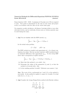
be expressed by Eq. (58). For other values of L, the dependence could best be
given by15
14
15
For σ not equal to 0.71, it is recommended that the factor 0.94 be replaced by ( 0.76σ −0.6 ).
Note that Lees [see reference 7, Eq. (19)] suggested that, for the frozen boundary layer, the
18
Nu / Re
= 1 + ( L0.63 − 1)
( Nu / Re ) L =1
hD
.
hs
(65)
The calculated values are compared with Eq. (65) in Fig. 4.
The difference in the exponent of L for the frozen as compared with the
equilibrium boundary layer [Eqs. (60) and (65)] is quite certain since exactly the
same property variations were used in both cases, and also seems reasonable in
exponent of L in Eq. (65) be 2/3.
19
view of the greater importance of diffusion throughout the whole of the frozen
boundary layer. It can be seen, however, that for a Lewis Number not too far
from unity there is little difference in heat transfer for the frozen as opposed to
the equilibrium boundary layer.
A few cases for noncatalytic wall were also computed. The resultant
heat-transfer parameter could be given approximately by Eq. (62) with L = 0 -i.e., the heat transfer becomes proportional to hs − hD .
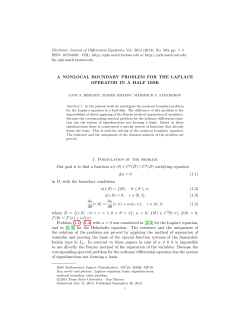
A comparison of the distributions of enthalpy, temperature, and atom
concentration for an equilibrium and a frozen boundary layer with identical
catalytic wall and free-stream conditions is shown in Figs. 5 and 6. Both cases
give very nearly the same heat transfer; however, the enthalpy distributions are
slightly different (since L = 1.4) and the temperature and concentration
distributions are markedly different, as is the mechanism of heat transfer.
(10) FINITE RECOMBINATION RATE
This most general case was solved using Method 2 with values of the
recombination rate parameter ( C1 ) varying from zero (frozen) to infinity
(equilibrium). As for the frozen boundary layer, the wall may be either catalytic
or noncatalytic, and both of these alternatives were calculated. It is to be
expected, of course, that for large values of C1 (near equilibrium) there should
be little effect of wall catalysis, since few atoms reach the wall.
The heat-transfer parameter for one flight condition and wall temperature is
20
plotted in Fig. 7 for the complete range of C1 . The solid lines are the total heat
transfer for both catalytic (upper curve) and noncatalytic (lower curve) surfaces.
For the catalytic wall, the fraction of heat transfer by conduction alone is shown
by the dotted curve, so that the freezing of the boundary layer as recombination
slows down ( C1 decreasing) is easily evident.
For either wall condition, C1 must change by a factor of 10 4 in order for
the boundary layer to change from substantially frozen to equilibrium
throughout. Within this region of variation of C1 , the boundary layer will be
partly frozen (near the outer edge) and partly in equilibrium (near the wall).
Since the recombination term [Eq. (56)] varies as T −3.5 , and the temperature
changes by a factor of twenty between wall and external flow for the case
considered, large variations in the recombination rate are possible across the
boundary layer, thus permitting it to be partly frozen and partly in equilibrium.
For the noncatalytic wall, the distributions of atom mass fraction for several
21
recombination rate parameters are shown in Fig. 8. For C1 very large, no
atoms reach the wall, all having recombined in the gas. For lower values of C1 ,
some atoms reach the wall and, because none recombine on the wall, a finite
atom concentration builds up. For C1 approaching zero, there is no
recombination and hence no concentration gradients exist.
It can be seen in Fig. 7 that a much lower value of C1 is necessary to
“freeze” the boundary layer when a noncatalytic wall is used than would be the
case otherwise. This is caused by the “damming up” of the atoms at the
noncatalytic wall, resulting in greater recombination because of high local
concentrations.
From Eqs. (57) and (63) it can be seen that, for a given flight velocity (hence
Ts ), C1 varies as the square of the stagnation point density (and thus for
strong shock waves, as the square of the ambient density), and also as the nose
radius. Thus the boundary layer would become frozen at a high enough altitude,
this altitude being less for small nose radii than for large. In order to change
from a frozen to an equilibrium boundary layer, C1 must change by 10 4 , and
thus the density by 10 2 , which is an altitude change of about 100,000 ft.
(11) CONCLUSIONS
The laminar stagnation point heat transfer in dissociated air can be given by
Eqs. (63) and (65) for the equilibrium and frozen boundary layers, respectively.
These results were computed for a Prandtl Number of 0.71 and for a Lewis
Number which was constant throughout the boundary layer.
The major deviation in the heat-transfer parameter from the low temperature,
perfect gas value is due to the variation of ρµ across the boundary layer. The
heat transfer [Eq. (63)] is mainly dependent upon the value of ρµ at the outer
edge of the boundary layer.
If the wall catalyzes atomic recombination, the total heat transfer is not
much affected by a nonequilibrium state of the boundary layer if the Lewis
Number is near unity.
If the wall is noncatalytic, the heat transfer may be appreciably reduced
when the boundary layer is frozen throughout -- i.e., when the recombination
reaction time becomes much longer than the time for a particle to diffuse
through the boundary layer. Since the ratio of these times depends upon altitude
and nose radius, there is a scale effect which determines the chemical state of
the boundary layer.
APPENDDIX. DETAILS OF THE NUMERICAL SOLUTIONS
22
Method 1.
The momentum equation for the stagnation point boundary layer is given by
Eq. (35) -- namely,
(lf ηη )η + ffηgh +
1 ρs
− fη 2 = 0 .
2 ρ
(A1)
If thermal diffusion is neglected (i.e., Li T = 0 ) then the energy equation in
terms of the enthalpy becomes, from Eq. (37),
l
l
σ gη + fgη + σ
η
∑
hi − hi 0
cis
( Li − 1) s iη = 0 ,
hs
η
(A2)
or
l
σ (1 + d ) gη + fgη = 0 ,
η
(A3)
where
d≡
∑
hi − hi 0
∂s i
c is
( Li − 1)
hs
∂g p
= ( L − 1)
∑
∂c
(hi − hi ) i
∂h p
(A4)
0
where the subscript p denotes that the differentiation is at constant pressure and
it is assumed Li = L = constant for all species.
In Method 1, which is suitable only for the equilibrium boundary layer, Eqs.
(A l) and (A3) were solved simultaneously with the boundary conditions
f(0)=0,
f η ( 0) = 0 ,
g ( 0) = g w ,
f η (∞) = 1 ,
g (∞ ) = 1 .
The functions l, ρ s / ρ and d were evaluated from the calculated equilibrium
properties of air(11) and by taking the viscosity to vary according to
Sutherland's formula [see Section (5) above]. For given external (stagnation
point) flow conditions these quantities were plotted as functions of g. For
numerical computation it was convenient to use analytic expressions of the
following form:
l≡
α
α
ρµ
= 1 − 2 ,
ρwµw
g
g
ρs
= 1 − γ 1 (1 − g ) − γ 2 (1 − g ) 4 ,
ρ
d = ( L − 1)
∑ (h
i
∂c
− hi 0 ) i = β1e − β 2 / g .
∂h p
(A5)
(A6)
(A7)
The constants α , γ , β in each expression were determined by fitting these
expressions to the equilibrium air calculations (see Fig. 1).
23
Numerical solutions for this problem were obtained on an IBM 650
computer. The method of solution was to pick values of
fηη (0) and
gη (0) and integrate the equations directly, recording the resultant asymptotic
values of fη and g for large values of η . After three such integrations an
interpolation will produce better values of
fηη (0)
and
gη (0) . The
interpolation procedure was repeated until the required conditions at “infinity”
were met -- i.e., fη → 1 and g → 1 . This interpolation was made an integral
part of the numerical program so by starting with three initial guesses for
fηη (0) and gη (0) the program would run automatically to completion.
It should be noted that Eqs. (A1) and (A3) are formally identical with the
stagnation point equations solved by Cohen and Reshotko(10) except for the
function d [Eq. (A4)]. If L = 1, however, d ≡ 0; thus by specifying L = 1,
σ = 1 , l = 1 and ρ s / ρ = g , the stagnation point solutions given by Cohen
and Reshotko could be duplicated. (A table giving the specific values of the
parameters for which solutions were obtained by the method described above
may be obtained directly from the authors.)
Method 2
This method is a more general formulation in that it allows computation of
the nonequilibrium boundary layer. As may be expected, however, it involves
more approximations than the rather straightforward procedure of Method 1.
In the nonequilibrium case, the concentration of the various species is not
determined by the enthalpy and the (known) pressure. It is necessary, therefore,
to add a continuity equation for each species.‘ Furthermore, it is convenient to
express the thermodynamic properties in terms of the temperature and the
concentrations of the species. The energy equation should, therefore, be written
in terms of the temperature. To make this problem tractable it was assumed that
air is a diatomic gas composed of “air” molecules and “air” atoms with
properties properly averaged between oxygen and nitrogen. The dissociation
energy of an air atom was taken to be the average dissociation energy in the
external flow [see Eq. (59)]. With this assumption the problem is reduced to the
simultaneous solution of three equations (momentum, energy and atom
concentration) and the thermodynamic properties are to be expressed in terms of
the temperature and atom concentration.
The momentum equation is still Eq. (A3), with
ρs 1+ cA
=
θ,
ρ 1 + c As
l≡
(A8)
1
ρµ
=
ρ w µ w 1 + c A
24
3/ 2
θw
F (θ ) ,
θ
(A9)
where
T θ
F (θ ) = s
300
2
3/ 2
4
Tθ
Tθ
413
+ 3.7 s − 2.35 s ,
Tsθ + 113
10
,
000
10,000
and the stagnation temperature Ts is given in degrees Kelvin. The function
F (θ ) is a fitted curve giving the temperature dependence of the viscosity under
the assumption that the atoms and molecules have the same collision
cross-sections.
The energy equation in terms of the temperature is, from Eq. (36) with
T
Li = 0 ,
l
cl
σ θη + cfθη + σ θη
η
c pi
∑c
pw
du
Li cis s iη + 2 e
dx
s
−1
∑
wt hi 0 − hi
=0
ρ c pwTs
(A10)
where
c≡
cp
c pw
.
With the assumption of a simple diatomic gas and taking Li = L = constant , the
third term may be rewritten as
Ll
σ
θη c Aη
c pA − c pM
c pw
,
and the fourth term, using Eqs. (56), (57), and (61), and taking h A = hM ,
becomes
C1
hD c A 2 − c AE 2
.
c pwTs θ 3.5 (1 + c As )
Now
~
R
M
c pM ≈
7
− (T / T ) 2
+e V
2
where the exponential is the vibrational heat capacity and TV ≈ 800°K. for air;
also
c pA =
~
5 R
.
2 M /2
Hence,
c≡
cp
c pw
=
c pA − c pM
c pw
2
10
2
c A + 1 + e −(θV / θ ) (1 − c A ) ,
7
7
=
3 2 −(θV / θ ) 2
.
− e
7 7
(A11)
(A12)
For computation then the energy equation becomes
Ll
cl
σ θη + cfθη + e σ θη c Aη + C1C 2 m = 0 ,
η
25
(A13)
where
l≡
1
ρµ
=
ρ w µ w 1 + c A
e≡
c≡
c pA − c pM
c pw
cp
c pw
=
3/ 2
θw
F (θ ) , see Eq. (A9)
θ
3 2
= −
7 7
− (θV / θ ) 2
,
2
10
2
c A + 1 + e −(θV / θ ) (1 − c A ) ,
7
7
C1 = parameter, see Eq. (57),
C2 ≡
m≡
hD
= parameter, see Eq. (61),
c pwTs
c A 2 − c AE 2
θ 3.5 (1 + c A )
.
The equilibrium atom mass fraction c AE can be determined from reference 11.
For computation c AE was approximated by
c AE = c As e C3 (1−1 / θ ) ,
(A14)
where C3 is a constant.
The continuity equation for atoms was written in terms of the atom mass
fraction c A instead of the normalized atom mass fraction s. Thus Eq. (34)
becomes
du e
lL
σ c Aη + fc Aη − 2 dx
η
s
−1
wi
∑ρ
=0.
(A15)
or
lL
σ c Aη + fc Aη − C1m = 0 .
η
(A16)
Method 2 for the nonequilibrium boundary layer is the simultaneous solution
of Eqs. (A1), (A13) and (A16) with the boundary conditions
f (0) = 0 ,
f η ( 0) = 0 ,
θ ( 0) = θ w ,
θ (∞ ) = 1 ,
f η (∞ ) = 1 ,
c A (0) = 0 for catalytic wall, c Aη (0) = 0 for noncatalytic wall,
c A (∞) = c As .
Solutions were obtained on a digital computer using an iterative procedure
similar to that need in Method 1.
The limiting case of the equilibrium boundary layer was obtained by Method
2 by eliminating the term C1 m between Eqs. (A13) and (A16) and solving the
resulting equation simultaneously with Eq. (A1), taking the equilibrium atom
concentration as a known quantity in the form of Eq. (A14). The limiting case of
the frozen boundary was obtained by putting C1 ≡ 0 .16
16
Numerical results of these calculations may be obtained directly from the authors.
26
REFERENCES
1. Moore, L. L., A Solution of the Laminar Boundary Layer Equations for a
Compressible Fluid with Variable Properties, Including Dissociation, Journal of
the Aeronautical Sciences, Vol. 19, No. 8, pp. 505-515, August, 1952.
2. Hansen, C. F., Note on the Prandtl Number for Dissociated Air, Journal of the
Aeronautical Sciences, Vol. 20, No. 11, pp. 789-790, November, 1953.
3. Romig, M. F., and Dore, F. J., Solutions of the Compressible Laminar
Boundary Layer Including the Case of a Dissociated Free Stream, Convair
Report No. ZA-7-012, San Diego, Calif., 1954.
4. Beckwith, I. B., The Effect of Dissociation in the Stagnation Region of a
Blunt-Nosed Body, Journal of the Aeronautical Sciences, Vol. 20, No. 9, pp.
645-646, September, 1953.
5. Crown, J. C., The Laminar Boundary Layer at Hypersonic Speeds. Navord
Report 2299, U.S. Naval Ordnance Lab., 1952.
6. Mark, R., Compressible Laminar Heat Transfer Near the Stagnation Point of
Blunt Bodies of Revolution, Convair Report No. ZA-7-016, San Diego, Calif.,
1955.
7. Lees, L., Laminar Heat Transfer Over Blunt-Nosed Bodies at Hypersonic
Flight Speeds, Jet Propulsion, Vol. 26, No. 4, pp. 259-259, 1956.
8. Hirschfelder, J. O., Curtiss, C. F., and Bird, R. B., Molecular Theory of Gases
and Liquids, John Wiley and Sons, Inc., New York, 1954.
9. Probstein, R. F., Methods of Calculating the Eguilibrium Laminar Heat
Transfer Rate at Hypersonic Flight Speeds, Jet Propulsion, Vol. 26, No. 6, pp.
497-499, 1956.
10. Cohen, C. B., and Reshotko, B., Similar Solutions for the Compressible
Laminar Boundary Layer with Heat Transfer and Pressure Gradient, NACA TN
3325, 1955.
11. Hilsendrath, J. and Beckett, C., Tables of Thermodynamic Properties of
Argon-free
Air
to
15,000°K,
AEDC-TN-56-12,
Arnold
Engineering
Development Center, USAF, September. 1956 (ASTIA Document No.
AD-98974).
12. Fay, J. A., Riddell, F. R., and Kemp, N. H., Stagnation Point Heat Transfer in
Dissociated Air Flow, Technical Notes, Jet Propulsion, Vol. 27, pp. 672-674,
1957.
13. Fay, J. A., The Laminar Boundary Layer in a Dissociating Gas, Avco
Research Laboratory TM-13, June, 1955.
14. Kuo, Y. H., Dissociation Effects in Hypersonic Viscous Flows, Journal of the
Aeronautical Sciences, Vol. 24, No. 5, pp. 345-350, May, 1957.
27
15. Rose, P. H., and Stark, W. I., Stagnation Point Heat-Transfer Measurements
in Dissociated Air, Journal of the Aeronautical Sciences, Vol. 25, No. 2, pp.
86-97, Februry, 1958.
28
© Copyright 2026 ExpyDoc