Fire Dynamics
Simulator
Wolfram Jahn
Lulea, 13th -15th of March 2014
About FDS
Developed by Kevin McGrattan at NIST for examining fire and
smoke movement in enclosed spaces such as atria, exhibition
halls, warehouses, tunnels, etc
2
About FDS
Developed by Kevin McGrattan at NIST for examining fire and
smoke movement in enclosed spaces such as atria, exhibition
halls, warehouses, tunnels, etc
FDS consists of
− Navier-Stokes solver
About FDS
Developed by Kevin McGrattan at NIST for examining fire and
smoke movement in enclosed spaces such as atria, exhibition
halls, warehouses, tunnels, etc
FDS consists of
− Navier-Stokes solver
− Turbulence Model
About FDS
Developed by Kevin McGrattan at NIST for examining fire and
smoke movement in enclosed spaces such as atria, exhibition
halls, warehouses, tunnels, etc
− Navier-Stokes solver
− Turbulence Model
FDS consists of − Combustion Model
About FDS
Developed by Kevin McGrattan at NIST for examining fire and
smoke movement in enclosed spaces such as atria, exhibition
halls, warehouses, tunnels, etc
− Navier-Stokes solver
− Turbulence Model
FDS consists of − Combustion Model
− Radiation Model
About FDS
Developed by Kevin McGrattan at NIST for examining fire and
smoke movement in enclosed spaces such as atria, exhibition
halls, warehouses, tunnels, etc
− Navier-Stokes solver
− Turbulence Model
FDS consists of − Combustion Model
− Radiation Model
− Boundary heat transfer
About FDS
Navier-Stokes:
Mass Conservation
000
∂ρ
˙b
+ ∇ · ρu = m
∂t
Change of mass in
Control Volume
About FDS
Navier-Stokes:
Mass Conservation
000
∂ρ
˙b
+ ∇ · ρu = m
∂t
Incoming/Outgoing
mass
About FDS
Navier-Stokes:
Mass Conservation
000
∂ρ
˙b
+ ∇ · ρu = m
∂t
Produced mass
About FDS
Navier-Stokes:
Mass Conservation
000
∂ρ
˙b
+ ∇ · ρu = m
∂t
Momentum Conservation
∂ (ρu) + ∇ · ρuu + ∇p = ρg + f + ∇ · τ
b
ij
∂t
Change of momentum
in Control Volume
About FDS
Navier-Stokes:
Mass Conservation
000
∂ρ
˙b
+ ∇ · ρu = m
∂t
Momentum Conservation
∂ (ρu) + ∇ · ρuu + ∇p = ρg + f + ∇ · τ
b
ij
∂t
Inertia
About FDS
Navier-Stokes:
Mass Conservation
000
∂ρ
˙b
+ ∇ · ρu = m
∂t
Momentum Conservation
∂ (ρu) + ∇ · ρuu + ∇p = ρg + f + ∇ · τ
b
ij
∂t
Pressure difference
(external force)
About FDS
Navier-Stokes:
Mass Conservation
000
∂ρ
˙b
+ ∇ · ρu = m
∂t
Momentum Conservation
∂ (ρu) + ∇ · ρuu + ∇p = ρg + f + ∇ · τ
b
ij
∂t
Gravity
About FDS
Navier-Stokes:
Mass Conservation
000
∂ρ
˙b
+ ∇ · ρu = m
∂t
Momentum Conservation
∂ (ρu) + ∇ · ρuu + ∇p = ρg + f + ∇ · τ
b
ij
∂t
Some external force
About FDS
Navier-Stokes:
Mass Conservation
000
∂ρ
˙b
+ ∇ · ρu = m
∂t
Momentum Conservation
∂ (ρu) + ∇ · ρuu + ∇p = ρg + f + ∇ · τ
b
ij
∂t
Shear forces
About FDS
Navier-Stokes:
Mass Conservation
000
∂ρ
˙b
+ ∇ · ρu = m
∂t
Momentum Conservation
∂ (ρu) + ∇ · ρuu + ∇p = ρg + f + ∇ · τ
b
ij
∂t
Energy Conservation
∂ (ρh) + ∇ · ρhu = Dp + q˙ 000 − ∇ · q˙ 00
Dt
∂t
Change of energy in
Control Volume
About FDS
Navier-Stokes:
Mass Conservation
000
∂ρ
˙b
+ ∇ · ρu = m
∂t
Momentum Conservation
∂ (ρu) + ∇ · ρuu + ∇p = ρg + f + ∇ · τ
b
ij
∂t
Energy Conservation
∂ (ρh) + ∇ · ρhu = Dp + q˙ 000 − ∇ · q˙ 00
Dt
∂t
Incoming/Outgoing
energy by convection
About FDS
Navier-Stokes:
Mass Conservation
000
∂ρ
˙b
+ ∇ · ρu = m
∂t
Momentum Conservation
∂ (ρu) + ∇ · ρuu + ∇p = ρg + f + ∇ · τ
b
ij
∂t
Energy Conservation
∂ (ρh) + ∇ · ρhu = Dp + q˙ 000 − ∇ · q˙ 00
Dt
∂t
Pressure changes
About FDS
Navier-Stokes:
Mass Conservation
000
∂ρ
˙b
+ ∇ · ρu = m
∂t
Momentum Conservation
∂ (ρu) + ∇ · ρuu + ∇p = ρg + f + ∇ · τ
b
ij
∂t
Energy Conservation
∂ (ρh) + ∇ · ρhu = Dp + q˙ 000 − ∇ · q˙ 00
Dt
∂t
Energy production
About FDS
Navier-Stokes:
Mass Conservation
000
∂ρ
˙b
+ ∇ · ρu = m
∂t
Momentum Conservation
∂ (ρu) + ∇ · ρuu + ∇p = ρg + f + ∇ · τ
b
ij
∂t
Energy Conservation
∂ (ρh) + ∇ · ρhu = Dp + q˙ 000 − ∇ · q˙ 00
Dt
∂t
Incoming/Outgoing
energy by radiation
About FDS
Navier-Stokes:
Mass Conservation
000
∂ρ
˙b
+ ∇ · ρu = m
∂t
Momentum Conservation
∂ (ρu) + ∇ · ρuu + ∇p = ρg + f + ∇ · τ
b
ij
∂t
Energy Conservation
∂ (ρh) + ∇ · ρhu = Dp + q˙ 000 − ∇ · q˙ 00
Dt
∂t
Gas Equation (for closure)
p = ρRspec T
About FDS
•
FDS solves a simplified version of Navier-Stokes, appropiate
for slow, buoyancy driven flows.
About FDS
•
FDS solves a simplified version of Navier-Stokes, appropiate
for slow, buoyancy driven flows.
• Finite difference discretisation on a rectangular grid.
About FDS
•
FDS solves a simplified version of Navier-Stokes, appropiate
for slow, buoyancy driven flows.
• Finite difference discretisation on a rectangular grid.
• Large Eddy Simulation (or DNS if required) for turbulences:
About FDS
•
FDS solves a simplified version of Navier-Stokes, appropiate
for slow, buoyancy driven flows.
• Finite difference discretisation on a rectangular grid.
• Large Eddy Simulation (or DNS if required) for turbulences:
→ Large eddies are solved directly.
About FDS
•
FDS solves a simplified version of Navier-Stokes, appropiate
for slow, buoyancy driven flows.
• Finite difference discretisation on a rectangular grid.
• Large Eddy Simulation (or DNS if required) for turbulences:
→ Large eddies are solved directly.
→ Subscale eddies are approximated (Smagorinsky).
• Mixture fraction combustion model:
→ Infinite rate combustion.
• Two approaches to model a fire:
→ Prescribed HRR.
→ "Fire spread".
About FDS
•
Free (download it from https://code.google.com/p/fds-smv/).
About FDS
•
Free (download it from https://code.google.com/p/fds-smv/).
• Very easy to use (after this you’ll be ready to go).
About FDS
•
Free (download it from https://code.google.com/p/fds-smv/).
• Very easy to use (after this you’ll be ready to go).
• If used with caution, very powerful tool.
About FDS
•
Free (download it from https://code.google.com/p/fds-smv/).
• Very easy to use (after this you’ll be ready to go).
• If used with caution, very powerful tool.
• But potentially dangerous if miss-used, or used without
proper analysis of the results
About FDS
•
Free (download it from https://code.google.com/p/fds-smv/).
• Very easy to use (after this you’ll be ready to go).
• If used with caution, very powerful tool.
• But potentially dangerous if miss-used, or used without
proper analysis of the results
→ e.g. Sprinkler - Fire interaction DOES NOT WORK!!
Use FDS carefully...
•
Hundreds of parameters that can be adjusted.
Use FDS carefully...
•
Hundreds of parameters that can be adjusted.
• Most of them require advanced knowledge of fire dynamics and
numerical methods.
Use FDS carefully...
•
Hundreds of parameters that can be adjusted.
• Most of them require advanced knowledge of fire dynamics and
numerical methods.
• All of them come with a default.
Use FDS carefully...
•
Hundreds of parameters that can be adjusted.
• Most of them require advanced knowledge of fire dynamics and
numerical methods.
• All of them come with a default...so you don’t have to adjust them.
Use FDS carefully...
•
Hundreds of parameters that can be adjusted.
• Most of them require advanced knowledge of fire dynamics and
numerical methods.
• All of them come with a default...so you don’t have to adjust them.
• FDS offers many features that do not really work (fire spread,
sprinklers).
Use FDS carefully...
•
Hundreds of parameters that can be adjusted.
• Most of them require advanced knowledge of fire dynamics and
numerical methods.
• All of them come with a default...so you don’t have to adjust them.
• FDS offers many features that do not really work (fire spread,
sprinklers).
• There is no general grid convergence!!
• Non-physical phenomena are common, but are often not recognized.
→ Example: Burning at openings.
Use FDS carefully...
General Rule: GIGO!
Use FDS carefully...
General Rule: GIGO!
Garbage In – Garbage Out
How does FDS work?
FDS
How does FDS work?
Input file (plain text): MyModel.fds
FDS
How does FDS work?
Input file (plain text): MyModel.fds
Lots of time..
FDS
How does FDS work?
Input file (plain text): MyModel.fds
Lots of time..
FDS
How does FDS work?
Input file (plain text): MyModel.fds
Lots of time..
FDS
Output
(massive)
Creating an Input File
•
Plain text file. Any text editor will do..
Creating an Input File
•
Plain text file. Any text editor will do..
• Grid, geometry and boundary conditions are defined here.
Creating an Input File
•
Plain text file. Any text editor will do..
• Grid, geometry and boundary conditions are defined here.
• Use an existing input file rather than creating a new one
from scratch.
Creating an Input File
•
Plain text file. Any text editor will do..
• Grid, geometry and boundary conditions are defined here.
• Use an existing input file rather than creating a new one
from scratch.
• A valid line starts with an ’&’ – any line without it will not
be taken into account.
Creating an Input File
•
Plain text file. Any text editor will do..
• Grid, geometry and boundary conditions are defined here.
• Use an existing input file rather than creating a new one
from scratch.
• A valid line starts with an ’&’ – any line without it will not
be taken into account.
• A valid line has to finish with a ’\’.
Creating an Input File
CHID – Naming the input file:
// Setup of FDS file
&HEAD CHID=’First Example’, TITLE=’First Try’ /
Creating an Input File
The computational domain and grid:
// Setup of FDS file
&HEAD CHID=’First Example’, TITLE=’First Try’ /
// Grid spacing
&MESH IJK=120,192,40, XB=0.0,12.0,0.0,19.0,0.0,4.0 /
Creating an Input File
The computational domain and grid:
// Setup of FDS file
&HEAD CHID=’First Example’, TITLE=’First Try’ /
// Grid spacing
&MESH IJK=120,192,40, XB=0.0,12.0,0.0,19.0,0.0,4.0 /
X B = xi , xf , yi , yf , zi , zf
Creating an Input File
Simulation time:
// Setup of FDS file
&HEAD CHID=’First Example’, TITLE=’First Try’ /
// Grid spacing
&MESH IJK=120,192,40, XB=0.0,12.0,0.0,19.0,0.0,4.0 /
// Simulation time
&TIME T_END=10. /
Creating an Input File
Simulation time:
// Setup of FDS file
&HEAD CHID=’First Example’, TITLE=’First Try’ /
// Grid spacing
&MESH IJK=120,192,40, XB=0.0,12.0,0.0,19.0,0.0,4.0 /
// Simulation time
&TIME T_END=10. / if set to 0, only geometry is checked.
Creating an Input File
Miscellaneous:
// General Parameters
&MISC SURF_DEFAULT=’CONCRETE’, RADIATION=.FALSE.,TMPA=25.,
RESTART=.TRUE. /
Creating an Input File
Control:
// General Parameters
&MISC SURF_DEFAULT=’CONCRETE’, RADIATION=.FALSE.,TMPA=25.,
RESTART=.TRUE. /
// Control Parameters
&DUMP DT_RESTART=100.,NFRAMES=1800 /
Creating an Input File
Control:
// General Parameters
&MISC SURF_DEFAULT=’CONCRETE’, RADIATION=.FALSE.,TMPA=25.,
RESTART=.TRUE. /
// Control Parameters
&DUMP DT_RESTART=100.,DT_DEVC=5.,DT_SLCF=10. /
Defining the Geometry
Obstacles:
Walls, furniture, doors etc. are all defined using rectangle
blockages
Defining the Geometry
Obstacles:
Walls, furniture, doors etc. are all defined using rectangle
blockages
// Creating obstacles
&OBST XB=6.2,6.4,1.6,6.6,0.0,2.4 /
Defining the Geometry
Obstacles:
Walls, furniture, doors etc. are all defined using rectangle
blockages
// Creating obstacles
&OBST XB=6.2,6.4,1.6,6.6,0.0,2.4 /
from x
to x
Defining the Geometry
Obstacles:
Walls, furniture, doors etc. are all defined using rectangle
blockages
// Creating obstacles
&OBST XB=6.2,6.4,1.6,6.6,0.0,2.4 /
from y
to y
Defining the Geometry
Obstacles:
Walls, furniture, doors etc. are all defined using rectangle
blockages
// Creating obstacles
&OBST XB=6.2,6.4,1.6,6.6,0.0,2.4 /
from z
to z
Defining the Geometry
Boundary Conditions
•
The obstruction is a boundary condition to the flow (free slip)
Boundary Conditions
•
The obstruction is a boundary condition to the flow (free slip)
• What about thermal boundary conditions (to calculate heat
fluxes, wall temperatures)?
Boundary Conditions
•
The obstruction is a boundary condition to the flow (free slip)
• What about thermal boundary conditions (to calculate heat
fluxes, wall temperatures)?
Surfaces and Materials
&SURF ID=’Wall’,MATL_ID=’Paper’,’Concrete’,
THICKNESS=0.001,0.3,BACKING=’EXPOSED’/
Boundary Conditions
•
The obstruction is a boundary condition to the flow (free slip)
• What about thermal boundary conditions (to calculate heat
fluxes, wall temperatures)?
Surfaces and Materials
&SURF ID=’Wall’,MATL_ID=’Paper’,’Concrete’,
THICKNESS=0.001,0.3,BACKING=’EXPOSED’/
&MATL ID=’Paper’,CONDUCTIVITY=0.12,
SPECIFIC_HEAT=1.172,DENSITY=128./
&MATL ID=’Concrete’,CONDUCTIVITY=1.7,
SPECIFIC_HEAT=0.75,DENSITY=2400./
Boundary Conditions
•
SI units.
Boundary Conditions
•
SI units.
• Every Surface needs an ID associated to it.
Boundary Conditions
•
SI units.
• Every Surface needs an ID associated to it.
• Can be applied directly to an obstacle (all surfaces have
same ID).
Boundary Conditions
•
SI units.
• Every Surface needs an ID associated to it.
• Can be applied directly to an obstacle (all surfaces have
same ID).
• Or to a certain part of surface:
→ &VENT XB=6.2,6.2,1.6,6.6,0.0,2.4,SURF_ID=’WOOD’\
Boundary Conditions
•
SI units.
• Every Surface needs an ID associated to it.
• Can be applied directly to an obstacle (all surfaces have
same ID).
• Or to a certain part of surface:
→ &VENT XB=6.2,6.2,1.6,6.6,0.0,2.4,SURF_ID=’WOOD’\
• The BCs of the Computational domain have to defined:
Boundary Conditions
•
SI units.
• Every Surface needs an ID associated to it.
• Can be applied directly to an obstacle (all surfaces have
same ID).
• Or to a certain part of surface:
→ &VENT XB=6.2,6.2,1.6,6.6,0.0,2.4,SURF_ID=’WOOD’\
• The BCs of the Computational domain have to defined:
// All domain boundaries initially exposed
&VENT MB=’XMIN’,SURF_ID=’OPEN’/
&VENT MB=’XMAX’,SURF_ID=’OPEN’/
The Fire
•
Special case of Boundary Condition
The Fire
•
Special case of Boundary Condition
SURF ID
The Fire
•
Special case of Boundary Condition
SURF ID
• HRRPUA, RAMP
&SURF ID=’MyFire’,HRRPUA=700,RAMP_Q=’MyRamp’\
The Fire
•
Special case of Boundary Condition
SURF ID
• HRRPUA, RAMP
&SURF ID=’MyFire’,HRRPUA=700,RAMP_Q=’MyRamp’\
&RAMP ID=’MyRamp’,T=0,F=0.0/
The Fire
•
Special case of Boundary Condition
SURF ID
• HRRPUA, RAMP
&SURF ID=’MyFire’,HRRPUA=700,RAMP_Q=’MyRamp’\
&RAMP ID=’MyRamp’,T=0,F=0.0/
&RAMP ID=’MyRamp’,T=80,F=0.2/
The Fire
•
Special case of Boundary Condition
SURF ID
• HRRPUA, RAMP
&SURF ID=’MyFire’,HRRPUA=700,RAMP_Q=’MyRamp’\
&RAMP ID=’MyRamp’,T=0,F=0.0/
&RAMP ID=’MyRamp’,T=80,F=0.2/
&RAMP ID=’MyRamp’,T=120,F=0.5/
The Fire
•
Special case of Boundary Condition
SURF ID
• HRRPUA, RAMP
&SURF ID=’MyFire’,HRRPUA=700,RAMP_Q=’MyRamp’\
&RAMP
&RAMP
&RAMP
&RAMP
ID=’MyRamp’,T=0,F=0.0/
ID=’MyRamp’,T=80,F=0.2/
ID=’MyRamp’,T=120,F=0.5/
ID=’MyRamp’,T=150,F=1.0/
The Fire
•
Fuel is injected at such rate that, if burnt, produces HRRPUA.
The Fire
•
Fuel is injected at such rate that, if burnt, produces HRRPUA
• Adding HRRPUA and TMPIGN to any surface converts it into a fire
when TMPIGN is reached.
The Fire
•
Fuel is injected at such rate that, if burnt, produces HRRPUA
• Adding HRRPUA and TMPIGN to any surface converts it into a fire
when TMPIGN is reached.→Carful with that!
The Fire
•
Fuel is injected at such rate that, if burnt, produces HRRPUA
• Adding HRRPUA and TMPIGN to any surface converts it into a fire
when TMPIGN is reached.→Carful with that!
• Alternatively you can prescribe MLRPUA. This will produce injection
of gas at a rate of MLRPUA, which will burn if it finds adequate
conditions.
• A radially spreading fire can be prescribed by:
&VENT XB=0.0,5.0,1.5,9.5,0.0,0.0,SURF_ID=’FIRE’,
XYZ=1.5,4.0,0.0,SPREAD_RATE=0.03/
• You can also define pyrolysis parameters and get FDS to mimic a
"real" fire.
The Fire
•
Fuel is injected at such rate that, if burnt, produces HRRPUA
• Adding HRRPUA and TMPIGN to any surface converts it into a fire
when TMPIGN is reached.→Carful with that!
• Alternatively you can prescribe MLRPUA. This will produce injection
of gas at a rate of MLRPUA, which will burn if it finds adequate
conditions.
• A radially spreading fire can be prescribed by:
&VENT XB=0.0,5.0,1.5,9.5,0.0,0.0,SURF_ID=’FIRE’,
XYZ=1.5,4.0,0.0,SPREAD_RATE=0.03/
• You can also define pyrolysis parameters and get FDS to mimic a
"real" fire.→VERY Carful with that!
Other BCs
•
Mechanical ventilation (i.e. fancoils) can be modelled as air-flow
coming into or leaving the domain.
Other BCs
•
Mechanical ventilation (i.e. fancoils) can be modelled as air-flow
coming into or leaving the domain.
• The flow "disappears" ("appears") at the boundary.
Other BCs
•
Mechanical ventilation (i.e. fancoils) can be modelled as air-flow
coming into or leaving the domain.
• The flow "disappears" ("appears") at the boundary.
Air supply:
&SURF ID=’SUPPLY’, VEL=-1.2, COLOR=’BLUE’ /
&VENT XB=5.0,5.0,1.0,1.4,2.0,2.4, SURF_ID=’SUPPLY’ /
Other BCs
•
Mechanical ventilation (i.e. fancoils) can be modelled as air-flow
coming into or leaving the domain.
• The flow "disappears" ("appears") at the boundary.
Air supply:
&SURF ID=’SUPPLY’, VEL=-1.2, COLOR=’BLUE’ /
&VENT XB=5.0,5.0,1.0,1.4,2.0,2.4, SURF_ID=’SUPPLY’ /
Exhaust:
&SURF ID=’EXHAUST’, VEL=1.2, COLOR=’RED’ /
&VENT XB=5.0,5.0,1.8,3.3,2.0,2.4, SURF_ID=’EXHAUST’ /
Manage the Output
•
Point "measurements" are obtained by adding "measuring" Devices:
Manage the Output
•
Point "measurements" are obtained by adding "measuring" Devices:
→ &DEVC XYZ=2.0,6.4,0.0,QUANTITY=’TEMPERATURE’/
Manage the Output
•
Point "measurements" are obtained by adding "measuring" Devices:
→ &DEVC XYZ=2.0,6.4,0.0,QUANTITY=’TEMPERATURE’/
→ If a volume is given instead of a point, an integrated quantity is
recorded (HRR, Average Temperature)
Manage the Output
•
Point "measurements" are obtained by adding "measuring" Devices:
→ &DEVC XYZ=2.0,6.4,0.0,QUANTITY=’TEMPERATURE’/
→ If a volume is given instead of a point, an integrated quantity is
recorded (HRR, Average Temperature)
• Point "measurements" are recorded in spreadsheet format
(CHID_devc.csv)
• Devices (DEVC) can also be used to control actions:
→ Smoke detectors, Sprinklers etc.
• Add SETPOINT to DEVC line:
&DEVC XYZ=0,0,0,ID=’Clock’,QUANTITY=’TIME’,SETPOINT=30.,INITIAL_STATE=.TRUE./
Manage the Output
•
Point "measurements" are obtained by adding "measuring" Devices:
→ &DEVC XYZ=2.0,6.4,0.0,QUANTITY=’TEMPERATURE’/
→ If a volume is given instead of a point, an integrated quantity is
recorded (HRR, Average Temperature)
• Point "measurements" are recorded in spreadsheet format
(CHID_devc.csv)
• Devices (DEVC) can also be used to control actions:
→ Smoke detectors, Sprinklers etc.
• Add SETPOINT to DEVC line and link it to other item:
&DEVC XYZ=0,0,0,ID=’Clock’,QUANTITY=’TIME’,SETPOINT=30.,INITIAL_STATE=.TRUE./
&OBST XB=...,SURF_ID=’...’,DEVC_ID=’Clock’/
Manage the Output
•
Slice Files:
Manage the Output
•
Slice Files:
→ &SLCF PBZ=0.45,QUANTITY=’TEMPERATURE’,VECTOR=.TRUE./
Plane parallel to z = 0.45
Manage the Output
•
Slice Files:
→ &SLCF PBZ=0.45,QUANTITY=’TEMPERATURE’,VECTOR=.TRUE./
Manage the Output
•
Slice Files:
→ &SLCF PBZ=0.45,QUANTITY=’TEMPERATURE’,VECTOR=.TRUE./
• Boundary Files:
Manage the Output
•
Slice Files:
→ &SLCF PBZ=0.45,QUANTITY=’TEMPERATURE’,VECTOR=.TRUE./
• Boundary Files:
→ &BNDF QUANTITY=’TEMPERATURE’/
Manage the Output
•
Slice Files:
→ &SLCF PBZ=0.45,QUANTITY=’TEMPERATURE’,VECTOR=.TRUE./
• Boundary Files:
→ &BNDF QUANTITY=’TEMPERATURE’/
→ Define BNDF_DEFAULT=.FALSE. on the MISC line in order to avoid
innecessary output.
Manage the Output
•
Slice Files:
→ &SLCF PBZ=0.45,QUANTITY=’TEMPERATURE’,VECTOR=.TRUE./
• Boundary Files:
→ &BNDF QUANTITY=’TEMPERATURE’/
→ Define BNDF_DEFAULT=.FALSE. on the MISC line in order to avoid
innecessary output.
→ Define BNDF_OBST=.TRUE. on an OBST line you want to see.
Manage the Output
•
Slice Files:
→ &SLCF PBZ=0.45,QUANTITY=’TEMPERATURE’,VECTOR=.TRUE./
• Boundary Files:
→ &BNDF QUANTITY=’TEMPERATURE’/
→ Define BNDF_DEFAULT=.FALSE. on the MISC line in order to avoid
innecessary output.
→ Define BNDF_OBST=.TRUE. on an OBST line you want to see.
• Information contained in the slice files can be exported into
spreadsheet format if required (using fds2ascii, which can be
downloaded from the FDS website).
Finally...
•
The last line in an FDSv5 input file is ’&TAIL/’:
Finally...
•
The last line in an FDSv5 input file is ’&TAIL/’:
&OBST XB=5.6,6.2,5.8,6.6,0.0,2.0,SURF_ID=’WALL’/
&OBST XB=5.4,6.2,1.6,5.8,0.0,2.0,SURF_ID=’WALL’/
&SURF ID=’WALL’, MATL_ID=’...’.../
&MATL ID=’...’..../
&SLCF PBZ=0.45,QUANTITY=’TEMPERATURE’,VECTOR=.TRUE./
&TAIL/
How to run FDS?
•
If you run OS X or GNU/Linux, open a terminal.
How to run FDS?
•
If you run OS X or GNU/Linux, open a terminal.
• If you run Windows, open cmd window.
How to run FDS?
•
If you run OS X or GNU/Linux, open a terminal.
• If you run Windows, open cmd window.
• Change directory to where your input file is (cd
/to/your/fds/example/path)
How to run FDS?
•
If you run OS X or GNU/Linux, open a terminal.
• If you run Windows, open cmd window.
• Change directory to where your input file is (cd
/to/your/fds/example/path)
• Once in your working directory run FDS by typing:
How to run FDS?
•
If you run OS X or GNU/Linux, open a terminal.
• If you run Windows, open cmd window.
• Change directory to where your input file is (cd
/to/your/fds/example/path)
• Once in your working directory run FDS by typing:
fds5 inputfile.fds
Let’s try...
© Copyright 2026 ExpyDoc