Computational modelling techniques
Exercise set 5
Solutions
1. The gross national product (GNP) represents the sum of consumption purchases of goods
and services, government purchases of goods and services, and gross private investment
(which is the increase in inventories plus buildings constructed and equipment acquired).
Assume that the GNP is increasing at the rate of 3% per year, and that the national debt is
increasing at a rate proportional to the GNP.
a) Construct a system of two ordinary differential equations modeling the GNP and
national debt.
𝑑𝐺𝑁𝑃
= 0.03 𝐺𝑁𝑃
𝑑𝑡
𝑑𝐷
= 𝑘 𝐺𝑁𝑃, 𝑘 > 0
𝑑𝑡
b) Solve the system in part a, assuming the GNP is M0 and the national debt is N0 at year
0.
For the GNP, we have to solve
𝑑𝐺𝑁𝑃
𝑑𝑡
= 0.03 𝐺𝑁𝑃, given that GNP(t0=0) = M0.
𝑖𝑛𝑡𝑒𝑔𝑟𝑎𝑡𝑖𝑜𝑛
𝑑𝐺𝑁𝑃
= 0.03𝑑𝑡 ��������� ln(𝐺𝑁𝑃) + 𝐶1 = 0.03𝑡 + 𝐶2 ⇔ ln(𝐺𝑁𝑃) = 0.03𝑡 + 𝐶
𝐺𝑁𝑃
At time t0=0 we get the equation
ln(𝐺𝑁𝑃) = 0.03𝑡0 + 𝐶 ⇒ 𝐶 = ln(𝑀0 )
Replacing the value of the constant C into the previous equation yields:
𝐺𝑁𝑃
� = 0.03𝑡 ⇔ 𝐺𝑁𝑃(𝑡) = 𝑀0 𝑒 0.03𝑡
ln(𝐺𝑁𝑃) = 0.03𝑡 + ln(𝑀0 ) ⇔ ln �
𝑀0
For the national debt D, we have to solve
𝑖𝑛𝑡𝑒𝑔𝑟𝑎𝑡𝑖𝑜𝑛
𝑑𝐷
𝑑𝑡
𝑑𝐷 = 𝑘𝑀0 𝑒 0.03𝑡 𝑑𝑡 ��������� 𝐷 + 𝐶1 =
At time t0=0 we get the equation
𝑁0 =
= 𝑘𝐺𝑁𝑃, given that D(t0=0)=N0.
𝑘𝑀0 0.03𝑡
𝑘𝑀0 0.03𝑡
𝑒
+ 𝐶2 ⇔ 𝐷 =
𝑒
+𝐶
0.03
0.03
𝑘𝑀0 0.03𝑡
𝑘𝑀0
0 + 𝐶 ⇒𝐶 = 𝑁 −
𝑒
0
0.03
0.03
Replacing the value of the constant C into the previous equation yields:
𝐷(𝑡) =
𝑘𝑀0 0.03𝑡
(𝑒
− 1) + 𝑁0
0.03
c) Does the national debt eventually outstrip the GNP? Consider the ratio of the
national debt to the GNP.
If the national debt is to outstrip the GNP, we get:
𝐷(𝑡) > 𝐺𝑁𝑃(𝑡) ⇔
𝑘𝑀0 0.03𝑡
(𝑒
− 1) + 𝑁0 > 𝑀0 𝑒 0.03𝑡 ⇔
0.03
𝑘𝑀0 (𝑒 0.03𝑡 − 1) > 0.03(𝑀0 𝑒 0.03𝑡 − 𝑁0 ) ⇔ (𝑘 − 0.03)𝑀0 𝑒 0.03𝑡 > 𝑘𝑀0 − 0.03𝑁0
If the ratio k satisfies k > 0.03, then the relation above is equivalent to
𝑘𝑀0 − 0.03𝑁0
𝑒 0.03𝑡 >
(𝑘 − 0.03)𝑀0
so we can conclude that national debt eventually outstrips the GNP in this case. If we
have k = 0.03, we obtain
0 > 𝑘𝑀0 − 0.03𝑁0 = 0.03(𝑀0 − 𝑁0 )
and in this case the debt is larger than the GNP only if this was also the case in year
0. For k < 0.03 we must have
𝑒 0.03𝑡 <
𝑘𝑀0 − 0.03𝑁0
.
(𝑘 − 0.03)𝑀0
If the right hand side is negative, the inequality can never hold. If it is positive, it is
still a constant and in the long run the inequality becomes false, which means that
GNP will become greater than D even if it starts smaller.
2. For the differential equation
𝑑𝑦
𝑑𝑥
= (𝑦 − 1)(𝑦 − 2)(𝑦 − 3) identify the equilibrium values.
Which are stable and which are unstable?
𝑑𝑦
𝑑𝑥
The equilibrium points are given by solving the equation
equilibrium points: y1=1, y2=2, and y3=3.
= 0, so we get three
To identify the behavior around the equilibrium points, we need to establish the sign of the
𝑑2 𝑦
function (𝑦 − 1)(𝑦 − 2)(𝑦 − 3), then solve 𝑑𝑥 2 = 0 and establish its sign.
y’<0
y’>0
y’<0
y’>0
y
1
2
3
𝑑2 𝑦
= (𝑦 3 − 6𝑦 2 + 11𝑦 − 6)′ = (3𝑦 2 − 12𝑦 + 11)(𝑦 − 1)(𝑦 − 2)(𝑦 − 3)
𝑑𝑥 2
𝑑2 𝑦
√3
= 0 ⇔ 𝑦 ∈ {2 ± , 1, 2, 3}
2
3
𝑑𝑥
Decreasing
concave
function
Increasing function;
concavity changes
convex to concave
y’<0
y’>0
y’’<0
y’’>0
Increasing convex
function
Decreasing function;
concavity changes
convex to concave
y’<0
y’’<0
y’’>0
y’>0
y’’<0
y’’>0
y
1
2-√3/3
2
2+√3/3
3
The points y1=1 and y3=3 are unstable equilibrium points, and y2=2 is stable.
3. Consider two species whose survival depends on their mutual cooperation. An example
would be a species of bee that feeds primarily on the nectar of one plant species and
simultaneously pollinates the plant. One simple model of this mutualism is given by the
autonomous system
𝑑𝑥
= −𝑎𝑥 + 𝑏𝑥𝑦
𝑑𝑡
𝑑𝑦
= −𝑚𝑦 + 𝑛𝑥𝑦
𝑑𝑡
a) What assumptions are implicitly being made about the growth of each species in the
absence of cooperation?
In absence of cooperation, both species would decline up to eventual extinction.
b) Interpret the constants a, b, m and n in terms of the physical problem.
a and m are the decay rates for the two species. b and n represent the positive effect
of one species on the other.
c) What are the equilibrium levels?
𝑑𝑥
= 0 ⇔ −𝑎𝑥 + 𝑏𝑥𝑦 = 0 ⇔ 𝑥(𝑏𝑦 − 𝑎) = 0
𝑑𝑡
𝑑𝑦
= 0 ⇔ −𝑚𝑦 + 𝑛𝑥𝑦 = 0 ⇔ 𝑦(𝑛𝑥 − 𝑚) = 0
𝑑𝑡
𝑚 𝑎
𝑛 𝑏
The two equilibrium points are (0, 0) and � , �.
d) Perform a graphical analysis and indicate the trajectory directions in the phase plane.
𝑎
𝑑𝑥
≥ 0 ⇔ −𝑎𝑥 + 𝑏𝑥𝑦 ≥ 0 ⇔ 𝑦 ≥
𝑏
𝑑𝑡
y
𝑚
𝑑𝑦
≥ 0 ⇔ −𝑚𝑦 + 𝑛𝑥𝑦 ≥ 0 ⇔ 𝑥 ≥
𝑛
𝑑𝑡
𝑎
𝑏
𝑚
𝑛
e) Interpret the outcomes predicted by your graphical analysis. Do you believe the
model is realistic? Why?
𝑎
𝑚
When either of the two species is under the threshold ( or respectively), due to
𝑏
𝑛
the mutual cooperation between species, also the other population will be driven
down, leading eventually to the extinction of the two species.
When either one of the two populations is above the corresponding threshold, due
to the mutualism the other species will also increase, leading to infinite growth.
The model reflects well mutual cooperation among two species, but it is not realistic
in predicting infinite growth. A maximum supported population factor should be
introduced for both species.
4. In the model for the arms race (see course 11, slides 23-25), assume that an-bm<0, so the
equilibrium point lies in a quadrant other than the first one in the phase plane. Sketch the
lines dx/dt=0 and dy/dt=0 in the phase plane and label them and their intercepts on the
coordinate axes. Perform a graphical stability analysis to respond to the following:
Model:
𝑑𝑥
= −𝑎𝑥 + 𝑏𝑦 + 𝑐
𝑑𝑡
𝑑𝑦
= 𝑚𝑥 − 𝑛𝑦 + 𝑝
𝑑𝑡
To find the equilibrium point, the above derivatives should both be zero. We obtain the
𝑏𝑝+𝑐𝑛
𝑎𝑝+𝑐𝑚
,
�. To decide where this point is located in the plane, we
equilibrium point �
𝑎𝑛−𝑏𝑚 𝑎𝑛−𝑏𝑚
use the hypothesis an-bm<0 and also we assume that, since the signs of each term were
chosen to characterize the intuitive behavior of the model, the constants involved in the
model are all positive.
To draw the two lines, we find their intersection with the axes and plot the corresponding
points according to their sign. Next, we need to distinguish, for each line, the semi-plane that
makes the corresponding equation positive and the one that makes it negative. For this, it is
enough to plug the point (0, 0) in both equation and see that the result is positive for both
lines.
y
�−
𝑝
�0, �
𝑛
𝑝
, 0�
𝑚
A
B
𝒅𝒙
=𝟎
𝒅𝒕
D
C
𝒅𝒚
=𝟎
𝒅𝒕
Region A:
𝑑𝑥
𝑑𝑡
> 0,
𝑑𝑦
𝑑𝑡
<0
𝑐
�0, − �
𝑏
𝑐
� , 0�
𝑎
x
Region B:
Region C:
Region D:
𝑑𝑥
𝑑𝑡
𝑑𝑥
𝑑𝑡
𝑑𝑥
𝑑𝑡
> 0,
< 0,
< 0,
𝑑𝑦
𝑑𝑡
>0
𝑑𝑦
𝑑𝑡
<0
𝑑𝑦
𝑑𝑡
>0
a) Do any potential equilibrium levels for defense spending exist? List any such points
and classify them as stable or unstable.
𝑏𝑝+𝑐𝑛
𝑎𝑝+𝑐𝑚
The only possible equilibrium point is �
,
� which due to the sign of an𝑎𝑛−𝑏𝑚 𝑎𝑛−𝑏𝑚
bm is negative, and thus not viable for our defense spending model.
The equilibrium point is unstable. If we take for example a trajectory that starts in
region A, it will move downwards and to the right toward the equilibrium point. As it
approaches the equilibrium point, the derivatives dx/dt and dy/dt approach 0.
Depending on where the trajectory begins and the sizes of the constants a, b, c, m, n,
p, either the trajectory will continue moving downward into region D (and then move
away from the equilibrium point), or continue moving rightward into region B (and
again move away from the equilibrium point).
b) What outcome for defense spending is predicted by your graphical analysis?
Since defense expenses are positive, the initial values will correspond to a point in
region B (most probable), A or C (if one of the countries spends a lot more than the
other. In any case, according to this model, both countries will infinitely increase
their defense expenses.
5. Find the local minimum value of the function
𝑓(𝑥, 𝑦) = 𝑥𝑦 − 𝑥 2 − 𝑦 2 − 2𝑥 − 2𝑦 + 4
Calculate the critical point:
𝜕𝑓
= 𝑦 − 2𝑥 − 2 = 0
𝜕𝑥
𝜕𝑓
= 𝑥 − 2𝑦 − 2 = 0
𝜕𝑦
Check that the point (-2, -2) is a minimum: f(-2, -2)=0; f(-1,-1)=7 > f(-2, -2).
6. Find three numbers whose sum is 9 and whose sum of squares is as small as possible.
Let x, y and z be the two numbers. We need to minimize 𝑓(𝑥, 𝑦, 𝑧) = 𝑥 2 + 𝑦 2 + 𝑧 2 in such a
way that x+y+z=9. We can use the Lagrange multiplier merit function:
𝐿(𝑥, 𝑦, 𝑧, λ) = 𝑥 2 + 𝑦 2 + 𝑧 2 + λ(𝑥 + 𝑦 + 𝑧 − 9)
Minimize 𝐿(𝑥, 𝑦, 𝑧, λ)
𝜕𝐿
= 2𝑥 + λ = 0
𝜕𝑥
𝜕𝐿
= 2𝑦 + λ = 0
𝜕𝑦
𝜕𝐿
= 2𝑧 + λ = 0
𝜕𝑧
𝑥 = 3; 𝑦 = 3; 𝑧 = 3; λ = −6
𝛿𝐿
=𝑥+𝑦+𝑧−9=0
𝛿λ
𝑓(𝑥, 𝑦, 𝑧) = 27. If we vary 𝑥, 𝑦, 𝑧 we get for example 𝑓(2, 3, 4) = 29 > 27, so (3, 3, 3) is
indeed a minimum point.
© Copyright 2026 ExpyDoc