Solved with COMSOL Multiphysics 4.4
Anisotropic Heat Transfer through
W o v e n C a r bo n Fi b ers
Introduction
Composite materials like carbon-fiber-reinforced polymer (CFRP) have outstanding
properties. It is a lightweight material with high stiffness and high temperature
tolerance and therefore used in aerospace industry, civil engineering and also for
high-end sports goods.
Carbon crystals form flat ribbons. Large numbers of these ribbons are bundled
together and woven in different structures as required by the application area. The
bundles have anisotropic material properties. For thermal properties this means that
the thermal conductivity along the fiber axis is much higher than perpendicular to it.
In COMSOL Multiphysics, implementing anisotropic properties is straightforward in
the global coordinate system, which is set by default. However, in the present case, an
anisotropic thermal conductivity needs to be defined along woven fibers where the
global coordinate system is inapplicable. The curvilinear coordinate system provides
the possibility to create a coordinate system following the curves of a geometry in
which anisotropic material properties or anisotropic physics can be defined.
This tutorial model shows how to use the curvilinear coordinates interface and how to
apply it to define anisotropic thermal conductivity.
Model Definition
The model represents a cutout of a carbon-fiber-reinforced polymer. The geometry
used in this case is shown in Figure 1. The fiber bundles have circular cross-sections
and are embedded in a matrix made of epoxy.
1 |
A N I S O T R O P I C H E A T TR A N S F E R T H R O U G H WO V E N C A R B O N F I B E R S
Solved with COMSOL Multiphysics 4.4
Infinite Domains
Carbon Fibers
Figure 1: Model geometry: fibers embedded in an epoxy matrix (hidden) with infinite
element domain.
The “infinite domains” truncate the geometry to model a few fibers only. With the
Heat Transfer Module you can assign them as Infinite Element Domains and thus
suppress boundary effects. Without the Heat Transfer Module the boundary
conditions at the outer side will affect the solution-in this case the maximum
temperature. Increase the number of fibers to reduce these effects.
MATERIAL PROPERTIES
The material properties are summarized in Table 1.
TABLE 1: MATERIAL PROPERTIES
2 |
MATERIAL PROPERTY
EPOXY
CARBON (CORE)
CARBON (INFINITE DOMAIN)
Thermal conductivity
0.2 W/(m·K)
{60,4,4} W/(m·K)
60 W/(m·K)
Density
1200 kg/m³
1500 kg/m³
1500 kg/m³
Heat Capacity
1000 J/(kg·K)
1000 J/(kg·K)
1000 J/(kg·K)
A N I S O T R O P I C H E A T TR A N S F E R T H R O U G H WO V E N C A R B O N F I B E R S
Solved with COMSOL Multiphysics 4.4
Note the syntax of the thermal conductivity for carbon (core). In the general case of
an anisotropic thermal conductivity it is a second order tensor. In our case the tensor
is diagonal.
k xx k xy k xz
k = k yx k yy k yz
k k k
zx zy zz
60 0 0
=
0 40
0 04
Note, that the conductivity is high in fiber direction and low in perpendicular
direction. The coordinate system used for k must then provide an x-component
following the shape of the fibers. The Curvilinear Coordinates interface provides the
possibility to create such a base vector system.
CURVILINEAR COORDINATES
Three predefined methods and a user-defined method are available to set up a
curvilinear coordinate system. Further details can be found in the COMSOL
Multiphysics Reference Guide in the The Curvilinear Coordinates Interface section.
Here you use the diffusion method which solves Laplace’s equation resulting in a
scalar potential. It is the same as solving the stationary heat transfer equation with
temperature boundary conditions resulting in a temperature gradient and forming the
first base vector of the new coordinate system. The second base vector is specified
manually and the cross-product of both forms the third base vector.
Figure 1 shows the base vector system for a single fiber:
3 |
A N I S O T R O P I C H E A T TR A N S F E R T H R O U G H WO V E N C A R B O N F I B E R S
Solved with COMSOL Multiphysics 4.4
:
Figure 2: Curvilinear coordinate system from diffusion method.
Alternatively the Flow Method is available, which results in a vector potential. This is
equivalent to solving Stokes flow (also known as creeping flow) where the obtained
velocity field forms the first base vector. The third option is to choose the Elasticity
Method for solving an eigenvalue problem.
If the Create base vector system check box is enabled the new curvilinear system is
available as input for the Coordinate System Selection drop-down menu and thus
providing new x-y-z coordinates.
BOUNDARY CONDITIONS
For the curvilinear coordinates interface, the inlet and outlet boundaries define the
direction of the first base vector. The heat transfer analogy consists in setting a high
temperature at the inlet and a low temperature at the outlet. All other boundaries are
thermally insulated walls.
For the heat transfer interface, a constant temperature boundary condition is set at the
outermost walls. A boundary heat source described with a Gaussian pulse in the center
of the geometry is applied and a convective cooling boundary condition on both sides.
4 |
A N I S O T R O P I C H E A T TR A N S F E R T H R O U G H WO V E N C A R B O N F I B E R S
Solved with COMSOL Multiphysics 4.4
INFINITE ELEMENTS
To truncate the geometry the Infinite Element Domain feature can be used. Boundary
conditions applied to these elements can be imagined as boundary conditions at an
infinite distance of the modeling domain. So it does not affect the solution of this
particular problem. This works by scaling the width of the domain to be much larger
than the original geometry.
Results and Discussion
From the Curvilinear Coordinates interface a new coordinate system is obtained as
depicted in Figure 1. The temperature distribution on the surface shows a high
temperature at the center where the maximum of the Gaussian function is located and
decreases with increasing distance from the center. The temperature drop to 293 K as
specified in the boundary conditions occurs mainly in the Infinite Element Domains.
Figure 3: Temperature distribution on the surface.
5 |
A N I S O T R O P I C H E A T TR A N S F E R T H R O U G H WO V E N C A R B O N F I B E R S
Solved with COMSOL Multiphysics 4.4
Figure 4 shows clearly that the heat spreads preferentially along the fiber axis.
Figure 4: Temperature at the center plane and fiber structure (gray).
Notes About the COMSOL Implementation
This tutorial model demonstrates how to use the Curvilinear Coordinate interface for
defining anisotropic thermal conductivity. Hence, the instructions focus on this part
and start with loading the file carbon_fiber_geometry.mph. The steps needed to
create this file are quite complex. This document will not go into details but provide a
short summary instead.
The geometry sequence calls geometry subsequences depending on the global
parameter q. The subsequences define different cross-sections and can be found under
the Global Definitions node. Call the elliptical cross-section with q = 1 and the
rectangular cross-section with q = 2.
All subsequent geometry features are based on these subsequences. Inside some of the
features, a selection of geometric entities is created automatically by activating the
Create Selections check box. Instead of selecting objects manually, these selections are
used as input in the following geometry node. This approach makes sure that all
6 |
A N I S O T R O P I C H E A T TR A N S F E R T H R O U G H WO V E N C A R B O N F I B E R S
Solved with COMSOL Multiphysics 4.4
geometry operations adapt and produce the desired geometry automatically, even if a
geometry parameter changes.
Selections are also used on the finalized geometry to ensure that physical properties are
assigned to the intended entities. These selections are defined under Component
1>Definitions. They are used to automatically set up boundary and domain conditions
as well as the mesh. The resulting model is consistent for any choice of parameters. The
extra time needed to set up this kind of geometry sequence and to define selections is
regained through an accelerated physics modeling and meshing process.
Model Library path: Heat_Transfer_Module/Tutorial_Models,_Conduction/
carbon_fibers_ied.mph
Modeling Instructions
Start with loading the model file that contains the geometry and selections used
throughout the modeling process.
1 From the File menu, choose Open.
2 Browse to the model’s Model Library folder and double-click the file
carbon_fibers_geom.mph.
COMPONENT 1
Add the Curvilinear Coordinates interface for the fibers.
GEOMETRY 1
On the Home toolbar, click Add Physics.
ADD PHYSICS
1 Go to the Add Physics window.
2 In the Add physics tree, select Mathematics>Curvilinear Coordinates (cc).
3 In the Add physics window, click Add to Component.
CURVILINEAR COORDINATES
1 In the Model Builder window, under Component 1 click Curvilinear Coordinates.
2 In the Curvilinear Coordinates settings window, locate the Domain Selection section.
3 From the Selection list, choose Fibers (Core).
7 |
A N I S O T R O P I C H E A T TR A N S F E R T H R O U G H WO V E N C A R B O N F I B E R S
Solved with COMSOL Multiphysics 4.4
4 Locate the Settings section. Select the Create base vector system check box.
According to Curvilinear Coordinates the second basis vector is specified manually.
The y-direction feels natural.
Coordinate System Settings 1
1 In the Model Builder window, under Component 1>Curvilinear Coordinates click
Coordinate System Settings 1.
2 In the Coordinate System Settings settings window, locate the Settings section.
3 From the Second basis vector list, choose y-axis.
Diffusion Method 1
1 On the Physics toolbar, click Domains and choose Diffusion Method.
Wall is the default boundary condition where the normal component of the vector field
is zero. The direction of the first basis vector is specified with inlet and outlet boundary
conditions. That way it points from inlet to outlet.
2 In the Diffusion Method settings window, locate the Domain Selection section.
3 From the Selection list, choose Fibers (Core).
Inlet 1
1 Right-click Component 1>Curvilinear Coordinates>Diffusion Method 1 and choose
Inlet.
2 In the Inlet settings window, locate the Boundary Selection section.
3 From the Selection list, choose Inlets.
Outlet 1
1 Right-click Diffusion Method 1 and choose Outlet.
2 In the Outlet settings window, locate the Boundary Selection section.
3 From the Selection list, choose Outlets.
Now, built a suitable mesh manually. Start with meshing the fibers.
MESH 1
Size
1 In the Model Builder window, expand the Component 1>Mesh 1 node, then click Size.
2 In the Size settings window, locate the Element Size section.
3 From the Predefined list, choose Fine.
4 On the Mesh toolbar, click Boundary and choose Free Triangular.
8 |
A N I S O T R O P I C H E A T TR A N S F E R T H R O U G H WO V E N C A R B O N F I B E R S
Solved with COMSOL Multiphysics 4.4
Free Triangular 1
1 In the Model Builder window, under Component 1>Mesh 1 click Free Triangular 1.
2 In the Free Triangular settings window, locate the Boundary Selection section.
3 From the Selection list, choose Inlets.
Distribution 1
1 Right-click Component 1>Mesh 1>Free Triangular 1 and choose Distribution.
2 In the Distribution settings window, locate the Edge Selection section.
3 From the Selection list, choose Inlet Edges.
4 Locate the Distribution section. In the Number of elements text field, type 2.
5 On the Mesh toolbar, click Swept.
Swept 1
1 In the Model Builder window, under Component 1>Mesh 1 click Swept 1.
2 In the Swept settings window, locate the Domain Selection section.
3 From the Geometric entity level list, choose Domain.
4 From the Selection list, choose Fibers (Core).
Distribution 1
1 Right-click Component 1>Mesh 1>Swept 1 and choose Distribution.
2 In the Distribution settings window, locate the Domain Selection section.
3 From the Selection list, choose Fibers (Core).
4 Locate the Distribution section. In the Number of elements text field, type 10.
9 |
A N I S O T R O P I C H E A T TR A N S F E R T H R O U G H WO V E N C A R B O N F I B E R S
Solved with COMSOL Multiphysics 4.4
5 Click the Build Selected button.
Convert the surface elements into triangles in order to use a free tetrahedral mesh for
the epoxy domain.
Convert 1
1 In the Model Builder window, right-click Mesh 1 and choose More
Operations>Convert.
2 In the Convert settings window, locate the Geometric Entity Selection section.
3 From the Geometric entity level list, choose Boundary.
4 From the Selection list, choose Fiber Walls.
Use a triangular mesh at the remaining core boundaries and extrude the resulting
boundary mesh into the infinite element domains.
5 On the Mesh toolbar, click Boundary and choose Free Triangular.
Free Triangular 2
1 In the Model Builder window, under Component 1>Mesh 1 click Free Triangular 2.
2 In the Free Triangular settings window, locate the Boundary Selection section.
3 From the Selection list, choose Epoxy Boundaries (Core).
10 |
A N I S O T R O P I C H E A T TR A N S F E R T H R O U G H WO V E N C A R B O N F I B E R S
Solved with COMSOL Multiphysics 4.4
Size 1
1 Right-click Component 1>Mesh 1>Free Triangular 2 and choose Size.
2 In the Size settings window, locate the Element Size section.
3 From the Predefined list, choose Extra fine.
4 On the Mesh toolbar, click Swept.
Swept 2
1 In the Model Builder window, under Component 1>Mesh 1 click Swept 2.
2 In the Swept settings window, locate the Domain Selection section.
3 From the Geometric entity level list, choose Domain.
4 From the Selection list, choose Infinite Element Domains.
Distribution 1
1 Right-click Component 1>Mesh 1>Swept 2 and choose Distribution.
2 In the Distribution settings window, locate the Distribution section.
3 In the Number of elements text field, type 3.
4 On the Mesh toolbar, click Free Tetrahedral.
Free Tetrahedral 1
Mesh the remaining part with a free tetrahedral mesh.
1 In the Model Builder window, under Component 1>Mesh 1 right-click Free Tetrahedral
1 and choose Build All.
11 |
A N I S O T R O P I C H E A T TR A N S F E R T H R O U G H WO V E N C A R B O N F I B E R S
Solved with COMSOL Multiphysics 4.4
The final mesh looks like this:
2 On the Home toolbar, click Add Study.
ADD STUDY
Add a stationary study to compute the new coordinate system with the Diffusion
Method.
1 Go to the Add Study window.
2 Find the Studies subsection. In the Select study tree, select Preset Studies>Stationary.
3 In the Add study window, click Add Study.
STUDY 1
Step 1: Stationary
On the Home toolbar, click Compute.
RESULTS
Coordinate System (cc)
The default plots show the coordinate system with volume arrows plots and a
streamlines plot for the vector field. To create the plot shown in Figure 3, add a
12 |
A N I S O T R O P I C H E A T TR A N S F E R T H R O U G H WO V E N C A R B O N F I B E R S
Solved with COMSOL Multiphysics 4.4
selection to the data set. The plot group then will use this subset of the whole
geometry only.
Data Sets
1 In the Model Builder window, expand the Results>Data Sets node.
2 Right-click Solution 1 and choose Add Selection.
3 In the Selection settings window, locate the Geometric Entity Selection section.
4 From the Geometric entity level list, choose Domain.
5 Click Paste Selection.
6 In the Paste Selection dialog box, type 20, 34, 54, 68, 88, 102, 122, 136 in
the Selection text field.
7 Click OK.
Coordinate System (cc)
1 In the Model Builder window, expand the Coordinate System (cc) node, then click First
Basis Vector.
2 In the Arrow Volume settings window, locate the Arrow Positioning section.
3 Find the x grid points subsection. In the Points text field, type 16.
4 Find the y grid points subsection. In the Points text field, type 2.
5 Find the z grid points subsection. In the Points text field, type 2.
6 In the Model Builder window, under Results>Coordinate System (cc) click Second Basis
Vector.
7 In the Arrow Volume settings window, locate the Arrow Positioning section.
8 Find the x grid points subsection. In the Points text field, type 16.
9 Find the y grid points subsection. In the Points text field, type 2.
10 Find the z grid points subsection. In the Points text field, type 2.
11 In the Model Builder window, under Results>Coordinate System (cc) click Third Basis
Vector.
12 In the Arrow Volume settings window, locate the Arrow Positioning section.
13 Find the x grid points subsection. In the Points text field, type 16.
14 Find the y grid points subsection. In the Points text field, type 2.
15 Find the z grid points subsection. In the Points text field, type 2.
16 On the 3D plot group toolbar, click Plot.
17 Click the Go to Default 3D View button on the Graphics toolbar.
13 |
A N I S O T R O P I C H E A T TR A N S F E R T H R O U G H WO V E N C A R B O N F I B E R S
Solved with COMSOL Multiphysics 4.4
Now add the Heat Transfer in Solids interface to the component.
ADD PHYSICS
1 Go to the Add Physics window.
2 In the Add physics tree, select Heat Transfer>Heat Transfer in Solids (ht).
3 In the Add physics window, click Add to Component.
H E A T TR A N S F E R I N S O L I D S
On the Physics toolbar, click Curvilinear Coordinates and choose Heat Transfer in Solids.
1 Click the Zoom Extents button on the Graphics toolbar.
2 On the Definitions toolbar, click Infinite Element Domain.
DEFINITIONS
Infinite Element Domain 1
1 In the Infinite Element Domain settings window, locate the Domain Selection section.
2 From the Selection list, choose Infinite Element Domains.
In order to apply a heat source right in the center of the model the Mass Properties
feature is used. It calculates the center of mass, which is automatically the center of the
geometry.
3 In the Model Builder window, right-click Definitions and choose Mass Properties.
4 In the Mass Properties settings window, locate the Source Selection section.
5 From the Selection list, choose Fibers (Core).
Define a heat source with the help of a local variable, which is defined on the boundary
only. Use the mass properties variable for the center of mass to apply the source term
exactly in the center.
Variables 1a
1 On the Home toolbar, click Variables and choose Local Variables.
2 In the Model Builder window, under Component 1>Definitions click Variables 1a.
3 In the Variables settings window, locate the Variables section.
14 |
A N I S O T R O P I C H E A T TR A N S F E R T H R O U G H WO V E N C A R B O N F I B E R S
Solved with COMSOL Multiphysics 4.4
4 In the table, enter the following settings:
Name
Expression
Unit
Description
Q_in
1e5[W/
m^2]*exp(-5e6[1/
m^2]*((x-mass1.CMx)
^2+(z-mass1.CMz)^2)
)
W/m²
Boundary heat source
In the next section, you define the materials according to the Material Properties
section.
MATERIALS
Material 1
1 On the Home toolbar, click New Material.
2 In the Material settings window, locate the Material Contents section.
3 In the table, enter the following settings:
Property
Name
Value
Unit
Property group
Thermal conductivity
k
0.2
W/(m·K)
Basic
Density
rho
1200
kg/m³
Basic
Heat capacity at constant pressure
Cp
1000
J/(kg·K)
Basic
4 Right-click Component 1>Materials>Material 1 and choose Rename.
5 In the Rename Material dialog box, type Epoxy in the New name edit field.
6 Click OK.
Material 2
1 On the Home toolbar, click New Material.
2 In the Material settings window, locate the Geometric Entity Selection section.
3 From the Selection list, choose Fibers.
4 Locate the Material Contents section. In the table, enter the following settings:
Property
Name
Value
Unit
Property group
Thermal conductivity
k
{60, 4, 4 }
W/(m·K)
Basic
Density
rho
1500
kg/m³
Basic
Heat capacity at constant
pressure
Cp
1000
J/(kg·K)
Basic
15 |
A N I S O T R O P I C H E A T TR A N S F E R T H R O U G H WO V E N C A R B O N F I B E R S
Solved with COMSOL Multiphysics 4.4
5 Right-click Component 1>Materials>Material 2 and choose Rename.
6 In the Rename Material dialog box, type Carbon in the New name edit field.
7 Click OK.
Material 3
1 On the Home toolbar, click New Material.
2 In the Material settings window, locate the Geometric Entity Selection section.
3 From the Selection list, choose Fibers (Infinite Element Domain).
4 Locate the Material Contents section. In the table, enter the following settings:
Property
Name
Value
Unit
Property group
Thermal conductivity
k
60
W/(m·K)
Basic
Density
rho
1500
kg/m³
Basic
Heat capacity at constant pressure
Cp
1000
J/(kg·K)
Basic
5 Right-click Component 1>Materials>Material 3 and choose Rename.
6 In the Rename Material dialog box, type Carbon (infinite element domain) in
the New name edit field.
7 Click OK.
Add a second Heat Transfer in Solids node for the fibers and choose the curvilinear
system as reference system. This way the thermal conductivity is high along the fiber
axis and low perpendicular to it.
H E A T TR A N S F E R I N S O L I D S
Heat Transfer in Solids 2
1 On the Physics toolbar, click Domains and choose Heat Transfer in Solids.
2 In the Heat Transfer in Solids settings window, locate the Domain Selection section.
3 From the Selection list, choose Fibers (Core).
4 Locate the Coordinate System Selection section. From the Coordinate system list,
choose Curvilinear System (cc).
5 Right-click Component 1>Heat Transfer in Solids>Heat Transfer in Solids 2 and choose
Rename.
6 In the Rename Heat Transfer in Solids dialog box, type Heat Transfer in fibers
in the New name edit field.
7 Click OK.
16 |
A N I S O T R O P I C H E A T TR A N S F E R T H R O U G H WO V E N C A R B O N F I B E R S
Solved with COMSOL Multiphysics 4.4
Set up the boundary conditions: the heat source, a convective heat-flux accounting for
cooling and a fixed temperature at the very outer boundaries of the infinite domain.
Boundary Heat Source 1
1 On the Physics toolbar, click Boundaries and choose Boundary Heat Source.
2 In the Boundary Heat Source settings window, locate the Boundary Selection section.
3 From the Selection list, choose Boundary Heat Source.
4 Locate the Boundary Heat Source section. In the Qb text field, type Q_in.
Convective Heat Flux 1
1 On the Physics toolbar, click Boundaries and choose Convective Heat Flux.
2 In the Convective Heat Flux settings window, locate the Boundary Selection section.
3 From the Selection list, choose Cooling Boundaries.
4 Locate the Heat Flux section. In the h text field, type 10.
Temperature 1
1 On the Physics toolbar, click Boundaries and choose Temperature.
2 In the Temperature settings window, locate the Boundary Selection section.
3 From the Selection list, choose Temperature Boundaries.
The first study was used to compute the curvilinear system. Add a second study to solve
for the heat transfer only. Refer to Study 1 in the Values of Dependent Variables section
by selecting the solution as input for the variables not solved in this second study. This
way the new coordinate system, which is initially unknown by Study 2, can be used for
the heat transfer calculation.
ADD STUDY
1 Go to the Add Study window.
2 Find the Studies subsection. In the Select study tree, select Preset Studies>Stationary.
3 Find the Physics in study subsection. In the table, enter the following settings:
Physics
Solve
Curvilinear Coordinates (cc)
×
4 In the Add study window, click Add Study.
17 |
A N I S O T R O P I C H E A T TR A N S F E R T H R O U G H WO V E N C A R B O N F I B E R S
Solved with COMSOL Multiphysics 4.4
STUDY 2
Step 1: Stationary
1 On the Home toolbar, click Add Study.
2 In the Model Builder window, under Study 2 click Step 1: Stationary.
3 In the Stationary settings window, click to expand the Values of dependent variables
section.
4 Locate the Values of Dependent Variables section. Select the Values of variables not
solved for check box.
5 From the Method list, choose Solution.
6 From the Study list, choose Study 1, Stationary.
7 On the Home toolbar, click Compute.
RESULTS
Temperature (ht)
The default temperature plot shows the temperature distribution on the surface
(Figure 3).
1 Click the Zoom Extents button on the Graphics toolbar.
To create Figure 4 follow the steps below:
Data Sets
1 In the Model Builder window, under Results>Data Sets right-click Solution 2 and
choose Duplicate.
2 Right-click Results>Data Sets>Solution 3 and choose Add Selection.
3 In the Selection settings window, locate the Geometric Entity Selection section.
4 From the Geometric entity level list, choose Domain.
5 From the Selection list, choose Core.
6 On the Results toolbar, click More Data Sets and choose Surface.
7 In the Surface settings window, locate the Data section.
8 From the Data set list, choose Solution 2.
9 Locate the Selection section. From the Selection list, choose Fiber Walls.
3D Plot Group 5
1 On the Home toolbar, click Add Plot Group and choose 3D Plot Group.
2 In the 3D Plot Group settings window, locate the Data section.
18 |
A N I S O T R O P I C H E A T TR A N S F E R T H R O U G H WO V E N C A R B O N F I B E R S
Solved with COMSOL Multiphysics 4.4
3 From the Data set list, choose Solution 3.
4 On the 3D plot group toolbar, click Slice.
5 In the Model Builder window, under Results>3D Plot Group 5 click Slice 1.
6 In the Slice settings window, locate the Expression section.
7 In the Expression text field, type T.
8 Locate the Plane Data section. From the Plane list, choose zx-planes.
9 In the Planes text field, type 1.
10 Locate the Coloring and Style section. From the Color table list, choose ThermalLight.
11 On the 3D plot group toolbar, click Surface.
12 In the Model Builder window, under Results>3D Plot Group 5 click Surface 1.
13 In the Surface settings window, locate the Expression section.
14 In the Expression text field, type 1.
15 Locate the Data section. From the Data set list, choose Surface 1.
16 Locate the Coloring and Style section. From the Coloring list, choose Uniform.
17 From the Color list, choose Gray.
18 Click the Go to ZX View button on the Graphics toolbar toolbar.
19 Click the Zoom Extents button on the Graphics toolbar toolbar.
20 In the Model Builder window, right-click 3D Plot Group 5 and choose Rename.
21 In the Rename 3D Plot Group dialog box, type Center temperature
distribution in the New name edit field.
22 Click OK.
19 |
A N I S O T R O P I C H E A T TR A N S F E R T H R O U G H WO V E N C A R B O N F I B E R S
Solved with COMSOL Multiphysics 4.4
20 |
A N I S O T R O P I C H E A T TR A N S F E R T H R O U G H WO V E N C A R B O N F I B E R S
© Copyright 2026 ExpyDoc