Automation, Control and Intelligent Systems 2014; 2(4): 42-52 Published online September 10, 2014 (http://www.sciencepublishinggroup.com/j/acis) doi: 10.11648/j.acis.20140204.11 ISSN: 2328-5583 (Print); ISSN: 2328-5591 (Online) Differential flatness applications to industrial machine control Ejike C. Anene1, Ganesh K. Venayagamoorthy2 1 2 Electrical Engineering Programme, Abubakar Tafawa Balewa University, PMB 0248, Bauchi, Nigeria Real-Time Power and Intelligent Systems Laboratory, Clemson University, Clemson, USA Email address: [email protected] (E. C. Anene), [email protected] (G. K. Venayagamoorthy) To cite this article: Ejike C. Anene, Ganesh K. Venayagamoorthy. Differential Flatness Applications to Industrial Machine Control. Automation, Control and Intelligent Systems. Vol. 2, No. 4, 2014, pp. 42-52. doi: 10.11648/j.acis.20140204.11 Abstract: In this article the applications of differential flatness to some industrial systems are presented. Computational methods of obtaining the flat output and the straight forward method of constructing the corresponding control law are given. Some theoretical and industrial systems are used as illustration including the third order synchronous machine model and the one degree of freedom magnetic levitation system model. Computations of the flat output are done using various approaches. The Levine’s approach is presented in such detail as to facilitate quick understanding. Computations for the synchronous machine model yielded a flat output that is a function of the load angle while the magnetic levitation model yielded a flat output that is a function of the objects’ position. Results showing the stabilization of the applied systems in fault and uncertain situations are discussed. Keywords: Magnetic Levitation, Flatness, Feedback Linearization, Synchronous Machine 1. Introduction THE concept of differential flatness proposed by Michel Fliess and co-workers [1],[2] about twenty years ago has evolved into a full-fledged field for the study of control systems in a practically new way. In this setting, controllability is linked with system flatness and controllable systems possess this flatness property [3],[4]. For such systems there is a solution set called flat output in the solution space consisting of a set of state variables that completely parameterize the system without the need for solving differential equations. Once this output is shown to be flat, it in effect implies that the system possesses a well characterized dynamics[5] . This is because all system parameters and control becomes a function of the linearizing output that can enable the generation of reference trajectories a-priori. The construction of the feedback law is done by a simple inversion of system equations with respect to the control. The scheme in derivation is an extension from the inputoutput linearization scheme with zero internal dynamics. Fliess et-al [1] proposed the notion of endogenous equivalence and defined a class of dynamic feedbacks for classification and linearization of systems in the form of Fliess’ differential algebraic forms. Such classes of systems are the so-called differentially flat systems. One of the main consequences of their result is a constructive method of computing the feedback that exactly linearizes a flat system. Accordingly a control system M , F is differentially flat around p if and only if it is equivalent to a trivial system in a neighborhood of p . A trivial system can be defined as one which is without dynamics described by a collection of independent variables or where Rs∞ , Fs Fs ( y , y (1) , y ( 2 ) ,.....) = ( y , y (1) , y ( 2 ) ,.....) , with y ⊂ R s y [6]. It is said to be differentially flat if it is differentially flat around every p of an open dense subset of M . The set y = { y j | j = 1,....., s} is called a flat or linearizing output of M described by a collection of independent variables, the flat output having the same number of components as the number of control variables. The following deductions are shown with proofs in [1]. 1. The number of components of a flat output is equal to number of input channels. 2. A classic linear system is flat if and only if it is controllable. 3. The controllability of differentially flat systems is related to the well known strong accessibility 43 Ejike C. Anene and Ganesh K. Venayagamoorthy: Differential Flatness Applications to Industrial Machine Control property of nonlinear systems due to Sussmann and Jurdjevic. 4. If a classic nonlinear system is differentially flat around p , then it satisfies the strong accessibility at p. 5. Differential flatness means that the state and input may be completely recovered from the flat output without integrating the system differential equations. After the introduction in Section 1, the paper discusses the basic theory of differential flatness in Section II. In Section III the procedure of computations of flat output is detailed. Section IV discusses the examples for computing flat outputs for some systems and the simulations done on the resulting controllers of some industrial systems on MATLAB. Conclusions are given in Section V while in Section VI the references are given. 2.1. Equivalence and Feedback The authors in [1] in their comprehensive paper unifying their theory of flatness and its associated dynamic feedback, formalized the concept that two systems are equivalent if there is an invertible transformation exchanging their trajectories, or if any variable of one system may be expressed as a function of the variables of the other system and of a finite number of their time derivatives. In a more general sense this transformation is said to be a LieBäcklund isomorphism. If two systems xɺ = f ( x , u),( x , u) ∈ X × U ⊂ R n × R m yɺ = g ( y , u),( y , v ) ∈ Y × V ⊂ R r × R s (6) and vector fields 2. Basic Theory of Flatness F ( x , u, u (1) , u ( 2 ) ....) = ( f ( x , u), u, u (1) , u ( 2 ) ....) A system variable is endogenous if it can be expressed as a linear combination of the input, the output and a finite number of their time derivatives. Otherwise it is exogenous. A single input single output (SISO) system is therefore flat or differentially flat if there exists an endogenous variable called the flat output, such that the input and the output can be expressed as a linear combination of the flat output and a finite number of its time derivatives [7]. Naturally any other endogenous variable of the system enjoys the same property with respect to the flat output. Thus the flat output differentially parameterizes all system variables. Generally, the definition of system flatness can be cast in what follows: The system G ( y , v , v (1) , v ( 2 ) ....) = ( g ( y , v), v, v (1) , v ( 2 ) ....) f ( xɺ, x , u) = 0 (1) with x ∈ R and u ∈ R is differentially flat if one can find a set of variables called flat output; n m y = h( x , u, uɺ, uɺɺ,....., u ( r ) ) (2) where, u = α ( x , z, w) zɺ = a ( x , z, w), with, z ∈ Z ⊂ R q f (0,0) = 0 (9) and rank (q) ) (3) ∂f (0,0) = m ∂u and control, u = β ( y , yɺ, ɺɺ,....., y y ( q +1) ) (4) with q a finite integer such that the system equation dα 0= f( ( y, yɺ , ɺyɺ,......, y ( q ) )), (5) dt (q) ( q +1) α ( y, yɺ , ɺyɺ,......, y ), β ( y, yɺ , ɺyɺ,......, y ) are identically satisfied [8]. (8) are differentially equivalent, it becomes possible to go from one to another by a dynamic feedback as shown in Figure 1. That is by a diffeomorphism of the extended state space X × Z . This dynamic feedback is endogenous if the original system is differentially equivalent to the closed loop system. It is called endogenous because the new z variables can be expressed as functions of the state and derivatives of the input. Thus from the work in [9] it can be stated that, if a system is differentially flat, there exists an endogenous dynamic feedback such that the closed loop system is diffeomorphic to a linear controllable system. Therefore for a nonlinear system equation (1), where y ∈ R m and system variables, x = α ( y , yɺ, ɺɺ,....., y y (7) (10) its dynamic feedback linearizability means the existence of: 1) dynamic compensator; zɺ = a ( x , z, v ), z ∈ R q u = b( x , z, v ), v ∈ R m where Automation, Control and Intelligent Systems 2014; 2(4): 42-52 a (0,0,0) = 0 b(0,0,0) = 0 2) xɺ = f ( x , b( x, z, v )) zɺ = β ( x , z, v ) (11) (13) u = α ( x, z, v) diffeomorphism; ξ = Ξ ( x, z),(ξ ∈ R n + q ) such that the 44 (12) and becomes a constant linear controllable system ξɺ = Fξ + Gv (n + q ) dimensional dynamics is given by (14) Figure 1. Transformation of a Nonlinear System into a Linear Equivalent. The components of u and x can be expressed as realanalytic functions of the component of equation (2), and a finite number of their derivatives (equations (3), (4)). The dynamic feedback is said to be endogenous if and only if the converse holds, that is, if and only if any component of y can be expressed as a real-analytic function of, x , u and a finite number of its derivatives. In a final remark in [1], the flat dynamics of a system whose output is given by equation (2) is square left and right input-output invertible system, where any component of u or x may, by definition be recovered from y without integrating any differential equation: It is said to possess a trivial zero-dynamics or a trivial residual dynamics. Figure 2 shows the endogenous dynamic feedback linearization process consisting of pole placement and linearization loops. 3.1. Classical Methods Following [4], consider a SISO system given by the transfer function y(s) = Ax + Bf = 0, B ≠ 0, rank [ A, B ] = n . (15) If A is invertible and B is full rank, then x solutions may be written in terms of f as x = − A−1 B f (16) and as such make all solutions parameterizable in terms of f . In this setting endogenous transformation ϕ in which the original variables of the system are transformed without creating new exogenous variables is realized [2]. (17) the system is controllable if and only if the polynomials n(s ) and d (s ) are coprime, that is they have no nontrivial common factors. By Bezout’s theorem, there exists polynomials a (s ) and b (s ) such that a ( s )n ( s ) + b( s )d ( s ) = 1 for all (18) s ∈ C . Define a new variable 3. Generating Flat Outputs Differential flatness is an idea that is naturally associated with underdetermined systems of differential equations where a system of n algebraic equations in n + m unknowns [4] is written as: n( s ) u (s) d (s) f (s) = 1 u( s) , d ( s) (19) we can write y ( s ) = n( s ) f ( s ) , u ( s ) = d ( s ) f ( s ) (20) multiplying both sides of (18) by f (s ) we have, a ( s ) n( s ) f ( s ) + b( s ) d ( s ) f ( s ) = f ( s ) or a ( s ) y ( s ) + b ( s )u ( s ) = f ( s ) (21) which implies we have a variable f which is a differential function of the system input and output and a finite number of their time derivatives. Conversely all system variables and input are also differential functions of the new variable. This new variable qualifies as a flat output. Therefore given any controllable linear system in transfer function 45 Ejike C. Anene and Ganesh K. Venayagamoorthy: Differential Flatness Applications to Industrial Machine Control form (17), the flat output can be chosen as any constant 1 multiple of the variable or f ( s) = u (s) d (s) k f ( s) = u ( s ) for any k ≠ 0 , for example consider the d (s) linear, coprime minimum phase function from (18), a( s )( s + 1) + b( s )( s − 1) = 1 s a ( s ) + a ( s ) + s b( s ) − b( s ) = 1 , satisfies a(s) = 1 2 y( s) = s +1 u ( s) s −1 , and b( s ) = − 1 2 the equation so that from (21), 1 1 . therefore parameterizes all system f f (s) = y( s) − u( s) 2 2 u ( s ) = d ( s ) f ( s ) = ( s − 1) f ( s ) = s f ( s ) − f ( s ) = fɺ − f similarly y ( s ) = n ( s ) f ( s ) = ( s + 1) f ( s ) = s f ( s ) + f ( s ) = fɺ + f This treatment can be extended to the state space approach [4]: For a given linear time-invariant SISO system described by y ( s) = bm s m + bm −1 s m −1 + ⋯ + b0 u ( s ), m < n s n + a n s n −1 + ⋯ + a0 (22) variables as given. Figure 2. Structure of Dynamic Feedback Linearization. with coprime polynomials in numerator and denominator κ admits a flat output f (s) = u ( s ) , which in n n −1 s + an s + ⋯ + a0 terms of differential equation and scalar output equation dn f gives: dt n + a n−1 d n−1 f dt n−1 + ⋯ + a0 f = κ u and −ke 1 L x1 + L u B x − 2 0 J JL2 JL2 JL F = ( 0 1) C x = ω C −1 = km km 0 x1 x1 ⋮ , y = c ⋮ A + bu x x n−1 n−1 x x n n 1 1 ⋯ 0 ⋮ ⋮ ⋱ ⋮ b = κ 0 0 ⋯ 1 1 − a1 ⋯ − an −1 R L2 1 L (24) , , are the controllability matrix, its Where , inverse and flat output respectively. The control is computed using as follows: 0 ⋯ 0) x1 = I = 1 ( J Fɺ + B F ) , km u = va = JL ɺɺ LB + RJ F + km km x2 = ω = F ɺ RB + ke F F + k m (25) 3.2. The Implicit Representation (Lévine’s Method) The flat output of such a system is given by f = (0,0,⋯1)(C ) −1 x where C = (b, Ab,⋯⋯, A n−1b) is the Kalman controllability matrix. Example: Given a DC motor dynamics [4] LIɺ + RI = va − keω J ωɺ + Bω = km I R xɺ1 − L = xɺ2 km J −1 x1 then d ⋮ = dt xn −1 x n κ R L2 km JL − km 1 dm f d m−1 f bm m + bm−1 m−1 + ⋯ + b0 f κ dt dt ɺ if x1 = f , x 2 = f ,…., x n = f (n ) y= 0 with ⋮ A= 0 − a 0 1 c = (b0 ⋯ bm 1 L C = 0 (23) where I=Armature current, w=Angular Velocity , , are are mechanical constants. electrical constants and , , The state space representation is given by Equation (1) can be locally transformed into an underdetermined implicit system F ( x , xɺ ) = 0 (26) for x ∈ X , and x, f ( x, u) ∈ Tx X ( Tangent space), for every u and rank df = m . This adopts a prolonged manifold of du solutions to the implicit representation. The author in [3] extends the notion of endogenous transformation (LieBäcklund Isomorphism) to the implicit system, stating that if two regular implicit systems of equation (6) are Lie- Automation, Control and Intelligent Systems 2014; 2(4): 42-52 Bäcklund equivalent then their linear cotangent approximation is locally Lie-Bäcklund equivalent. The Implicit system equation (26) is flat if and only if it is LieBäcklund equivalent. The system is flat if there exists local φ satisfying such that mappings φ ( y 0 ) = x0 Φ df i = 0 ; i = 1,....., n − m . * ∂F ∂F d Φ df = + ∂x ∂xɺ dt * dt diagonal reduction) given by (28) A matrix is M ∈ M p,q d is hyper-regular if and dt only if it’s Smith decomposition leads to I p , 0 p ,q − p , if p < q ; to 4. I P , if where id = 1 (−(ra + Re)(edn −V∞ sinδ) (ra + Re) + (xdn + xe )(xqn + xe) 2 + (xqn + xe )(eqn −V∞ cosδ)) iq = 1 (−( xdn + xe )(edn − V∞ sin δ ) (ra + Re )2 + ( xdn + xe )( xq + xe ) + (ra + Re )(eqn − V∞ cosδ )) 4.2. Implicit Method Using Lévine’s necessary and sufficient conditions for differential flatness [3] where for the system of equations (29) the system order n = 3 and the number of system input m = 1 . The notion of linear cotangent approximation henceforth called cotangent approximation is defined thus. Given a trajectory t ֏ x (t ) of (6)of class C VP ( F )U = ( ∆.θ n − m , m ) 3. δɺ = ω − ω 0 (27) where Φ*df = P(F ) , which are actually polynomial matrices and the differential operator d is the indeterminate. The dt inverse of a polynomial is not a polynomial and the inverse of a square matrix is not a matrix. These polynomial matrices have the following characteristics [3]: 1. They require the use of special algebraic manipulations. d 2. P ( F ) ∈ M n− m, n admits a Smith decomposition (or 46 p = q ; and to I p if p > q 0 p −q , q A square matrix M ∈ M p,q d is hyper-regular if dt and only if it is unimodular- denoted by u p d a dt subgroup of invertible matrices M d . p, q dt 5. P (F ) is hyper-regular if and only if the linear cotangent approximation of the implicit system equation (26) is controllable implying that the system is flat. These are the compact set of matrix manipulations that lead to the determination of the system’s flat output. 4. Application to Synchronous Machine 4.1. Synchronous Machine Reduced Order Model From the fourth order model of the synchronous ' machine , the direct axis e d can be assumed constant reducing it to a third order one-axis model [10] given by (29): τ d 0 eɺ q' = e fd − eq' − ( xd − xd' )id 2 H d 2δ = Pm − D(ω − ω 0 ) − ed' id − eq' iq wR dt 2 (29) interval J of ∞ on an ℜ , the linear time-varying implicit system ∂F ∂F ( x (t ), xɺ (t )) ξ (t ) + ( x (t ), xɺ (t )) ξɺ(t ) = 0 ∂x ∂xɺ (30) with ξ = (ξ ,ξɺ,...) ∈ ΤΧ , is defined as the linear cotangent approximation of equation (6) around the trajectory x . The system of equations (29) is first transformed to the implicit equivalent, obtained by eliminating the dynamics that contains the system input F (δ , ω , eq' , δɺ, ωɺ , eɺq' ) e fd , and making equal 0, Such that 2 H d 2δ − Pm + D(ω − ω 0 ) + ed' id + eq' iq = 0 ; w R dt 2 δɺ − ω + ω 0 = 0 (31) (32) The cotangent approximation to the implicit equations (31) and (32) is computed from: ∂F ∂F d ∂F ∂F d ∂F ∂F d P( F ) = + ɺ , + , ' + ' ∂δ ∂δ dt ∂ω ∂ωɺ dt ∂eq ∂eɺ q dt (33) It is noteworthy according to the characteristics above, that the cotangent approximation of system of equations (31) and (32) is hyper-regular if and only if it is controllable. And if it is locally flat around x 0 , its linear cotangent approximation around x 0 is controllable. Therefore there must exist V ∈ L − Smith ( P( F )) and U ∈ R − Smith ( P( F )) such that VP( F )U = ( I m , 0 n − m,m ) (34) The cotangent approximation after applying equation (33) on equation (31) and (32) yields: 47 Ejike C. Anene and Ganesh K. Venayagamoorthy: Differential Flatness Applications to Industrial Machine Control d dt a 21 −1 a 22 0 a 23 (35) where: a 21 = ω 0V ∞ 2 H det (eɺ (− R cosδ + x ' d e a 22 qt ) sin δ )δɺ + eq' ( xdt cosδ δɺ + Re cosδ ) ; P( F ) of rank n − m reduces to lower or upper triangular polynomial matrix to prove its hyper-regularity. The unimodular matrices are constructed in such a way to shuffle the elements of the cotangent approximation matrix and achieve lower triangular form. Successive steps of the reduction are given as follows [11]: Step a1: Multiplying equation (35) with the unimodular 0 1 0 matrix-1 1 0 0 gives d ω0 = + D ; dt 2 H 0 0 1 ω e' a 23 = 0 d ( x qt − x dt ) + V∞ ( x dt sin δ − Re cos δ ) + 2 ReV∞ eq' eɺ q' ; 2 H det d dt a21 and det = (ra + Re ) 2 + ( x d' + x e )( x q' + x e ) . 0 (36) a23 Step a2: Multiplying equation (36) with unimodular We now apply the Smith decomposition algorithm to equation (35) in successive polynomial matrix manipulations using unimodular matrices of rank n until d −1 dt d ω0 D a21 + dt 2 H d −1 0 1 0 −1 0 dt 1 0 0 = ω d a22 a23 0 0 1 + 0 D a21 dt 2 H d −1 0 dt 0 1 a23 0 0 matrix-2 d −1 dt 0 1 0 0 0 reduces 0 1 row 1 to [1 0 0] 0 1 0 0 = d ω0 d ω0 d − + D + D + a21 1 dt 2 H dt 2 H dt Step a3: Multiplying equation (37) with unimodular matrix -3 1 0 0 0 0 1 0 1 0 0 a23 (37) shuffles row 2 to make entry [2, 2] in (37) constant, yielding. 1 0 − d + ω0 D d + ω0 D d + a 21 dt 2 H dt 2 H dt 0 1 0 0 1 0 0 0 1 = d ω0 a23 D a23 − + 0 1 0 dt 2 H Step a4: Multiplying equation (38) with unimodular matrix-4 d ω0 d dt + 2 H D dt + a21 0 1 0 0 0 1 − 1 d + ω0 D d + a a23 a23 dt 2H dt 21 0 0 1 (38) achieves the required lower triangular matrix P (F ) . 1 0 ω d 0 − dt + 2 H D a23 Therefore 1 d ω0 d 0 dt + 2 H D dt + a21 0 1 0 0 P( F ) = − d + ω0 D 1 0 dt 2 H 0 0 1 a23 0 (40) Equation (40) which is a lower triangular polynomial matrix proves the hyper-regularity of equations (29). By right multiplying the unimodular matrices 1 to 4 used to generate P( F ) , the U matrix is generated as given in equations 41 to 43: Step b1: Unimodular matrix-1 by Unimodular matrix-2. 0 1 0 0 ω 1 d d 0 D + a21 = − d ω0 − + D 1 0 a23 dt 2 H dt + dt 2 H 1 0 0 0 1 0 − 1 1 0 dt d 0 1 0 0 0 1 0 = − 1 0 0 1 0 0 1 0 dt 0 1 (39) d (41) Step b2: Equation (41) by unimodular matrix-3 0 1 d −1 dt 0 0 0 0 1 1 0 0 0 0 0 0 1 = −1 0 0 1 0 0 1 1 d dt 0 (42) Automation, Control and Intelligent Systems 2014; 2(4): 42-52 dδ = dy Step 3 Equation (42) by unimodular matrix-4 0 0 −1 0 0 1 1 1 d 0 dt 0 0 0 0 = −1 0 1 0 a 23 1 1 d ω0 d − + + D a 21 a23 a23 dt 2 H dt 0 1 1 d dt 1 d ω0 d − + D + a21 a23 dt 2 H dt 0 0 1 d dt A33 Where A33 = − y=δ (43) Verification of the Flat Output of the Third Order SingleInput (SMIBS) model is done by showing that all the system states and variables are a function of the flat output and its derivatives. Thus from 1 d dt Uɵ = d 1 d ω0 − a ( dt + 2 H D) dt + a 21 23 (44) (45) (46) it is possible to compute by further matrix manipulations Q ∈ L − Smith (Uɵ ) which yields 1 d Q= − dt − A33 0 0 1 0 0 1 (47) where A33 is as defined above. Multiplying Q by the vector (dδ , dω , deq' ) T , the last two entries in the resulting vector d dδ + dω dt and 1 d ω0 d ( + D) + a 21 dδ + deq' dt a 23 dt 2 H which by (35) vanishes identically on X 0 . The first entry of the vector is therefore given by: (1 ωɺ = δɺɺ (51) and thus 1 1 R e '2 − (( x − x qt )ed' − V∞ ( − x dt sin δ − Re cos δ ))eq' − Pm det e q det dt (52) ed' 2 H ɺɺ δ=0 + D(ω − ω 0 ) + ( Re ed' + V∞ ( − Re sin δ − x qt cos δ )) + ω0 det Equation (52) is a quadratic function that can be ' evaluated for eq . Since the system states have been shown to be functions of the flat output and its derivatives, it follows that all other system variables which are functions of the states are also functions of the flat output and its derivatives. Hence: (53) 4.3. Compensator Design and Simulation Results 1 QUɵ = 0 0 − (50) ζ i = f i (δ , δɺ, δɺɺ) ∀ ζ i ∈ [ id , iq , vdt , vqt , Vt ] Using the definition are: ω = δɺ + ω 0 such that 1 d ω0 d ( + D) + a 21 . a 23 dt 2 H dt 0 2 ,1 Uɵ = U I1 (49) and so gives the flat output Equation (43) as U can be arranged compactly 0 0 U = −1 0 1 0 a 23 48 ( 0 0) dδ , dω , deq' ) T = dy Equation (48) is trivially strongly closed such that (48) It has been shown in the preceding section that the components of the system states and other system variables depending on the system states can be expressed as realanalytic functions of the component of δ and a finite number of its derivatives thus: x = A(δ , δɺ , δɺɺ) (54) The dynamic feedback is shown to be endogenous since the converse holds, that is, the flat output y is expressed as a real-analytic function of δ one of the states of the system. Thus the state of the SMIBS is a function of the linearizing output δ and its derivatives up to order α = 2 . The endogenous feedback system to the following closed loop system is of order α + 1 = 3 , so that from the linear system δɺɺɺ = v (55) the compensator follows. Considering the systems’ dynamical equations, perform the following state transformations: 49 Ejike C. Anene and Ganesh K. Venayagamoorthy: Differential Flatness Applications to Industrial Machine Control zɺ1 = z2 = yɺ 1 = δɺ = ω − ω 0 zɺ = z = ɺɺy = δɺɺ = ωɺ 2 3 (56) 1 ɺɺ = v zɺ 3 = ɺɺɺ y1 = δɺɺɺ = ω This yields the equivalent normal form for the system, from which we can compute the nonlinear controller by ɺɺ and inverting the expressions from ω . The state e fd Figure 3. Fault Location on the Single Machine Infinite Bus System (SMIBS) transformations are invertible and exist throughout the transient operating zone 0 < δ < 180 o . Using the network parameters of figure (3), the resulting excitation control is given by [11]: e fd = τ d0 2 H v Dωɺ + + Aeɺ 'd + Be 'd - Ce 'q + e 'q + (x d - x d' )i d (57) E detω 0 det where, A = 2R eT eɺ 'd - R eT V∞ sinδ - x qt V∞ cosδ ; B = x qt V∞ sin(δ )δɺ - R eT V∞ cos(δ )δɺ; C = (x dt - x qt )eɺ 'd - x dt V∞ cos(δ )δɺ - R eT V∞ sin(δ )δɺ ; E = (x dt - x qt )e 'd - x dt V∞ sinδ - 2R eT e 'q + R eT V∞ cosδ ; Figure 4. Responses of Speed Deviation to 3-Cycle Fault with and without FVDFC. and eɺ 'd = 1 ((x - x ' ) + x dt )(x dt cos(δ ) + R eT V∞ sin(δ )δɺ ) + ReT e 'q ; det q d ReT = (ra + Re ); x dt = ( x d' + x e ) ; x qt = ( x q' + x e ) e fd . is hereby proved also to be a function of the flat variable and its derivatives, that is e fd = β (δ , δɺ , δɺɺ) (58) The loop closure is then done to stabilize the system. v = − k1 (δ − δ 1* ) − k 2 (δɺ − δɺ1* ) − k 3 (δɺɺ − δɺɺ1* ) (59) and choose k i appropriately such that the linear time invariant error dynamics e ( 3) = k1e + k 2 eɺ + k 3 eɺɺ (60) where e ( j ) = δ ( j ) − (δ * ) ( j ) are stable. Equation (57) is the control law referred to as Field Voltage Dynamic Feedback Controller (FVDFC), [11] while (59) is the linear input that stabilizes the system to equilibrium. Simulation of the system was done by connecting the synchronous machine as a single machine infinite bus system (SMIBS) under a short circuit fault situation as shown in Figure 3. Figure 5. Responses of Terminal Voltage to 3-Cycle Fault with and without FVDFC. Some simulation results with the system equipped with the designed controller are presented in Figures 4 and 5 which are representative of the system performance. These figures clearly show the responses of the controller to a three-phase short circuit fault of 3-cycles duration. The system was restored to steady state operating point as the controller damped the fault oscillations under three seconds as shown by the machine speed deviation and the corresponding terminal voltage. The oscillations in the uncontrolled system were not damped within the same time duration. Automation, Control and Intelligent Systems 2014; 2(4): 42-52 50 Figure 6. Block diagram of INTECOTM maglev model The polynomial matrix will therefore be 5. Application to Magnetic Levitation The model development of the magnetic levitation is based on the system developed by INTECOTM for the purpose of teaching. The system block diagram is shown in Figure 6. INTECO used empirical analysis to model the control of the current that goes to the electromagnet. The resulting linear relationship is found to be a straight line i(u) = au + b with a dead zone. The constants a and b are determined from the experimental data. The system dynamics are described in (61) – (63). xɺ1 = x2 xɺ 2 = g − (61) 1 2 f _ p1 x3 m f _ p 2 xɺ 3 = ( k i u + c1 − x3 ) − x1 f_p 2 e (62) 1 − x1 p2 p1 e p2 (63) Where g is gravitational force, m is mass of object, f _ p1, f _ p2 , p1, p2 , ki , c1 are system constants. Flat output The flat output can be determined using Levine’s method by applying the implicit function theory and eliminating the dynamics with control. The variational equation is given by[12]: dɺxɺ1 − a e Where a= ( − x1 − x1 ) f −p f − p2 2 x3 dx1 − a e 2 x32 dx3 1 f _ p1 m f _ p2 2 d p( f ) = 2 − a e dt − x1 f _ p2 2 x3 dx1 dx 3 (65) or compactly dx1 p ( f ) = [ A − b] dx3 Where A= − x1 f _p 2 2 − a e x3 2 d2 dt - a (66) polynomial and − x1 f _ p 2 2 −a e x3 . Using Smith’s algorithm for the b= manipulation of polynomial matrices, the following right Smith steps are performed. [A 0 − b] 1 − b 1 1 A b 1 = [1 0] , therefore Uˆ = 1 A , such that b 0 1 1 = Q Uˆ = 1 1 0 A − b as required. (67) Therefore, 0 1 Q dx = 1 A − 1 b Such that the first line reads (64) − x1 f _ p 2 2 x3 − ae dx1 dx 3 dy = dx1 (68) which gives y = x1 the flat output, while the second line is identically equal to zero from (66) showing the flatness of the system dynamics. This follows that the flat output of this maglev model is the ball position which is also a system variable. 51 Ejike C. Anene and Ganesh K. Venayagamoorthy: Differential Flatness Applications to Industrial Machine Control a set point of 0.006 m. 5.1. Compensator Design and Simulation Results From the computed flat output the control law follow from the following compensator y = x1 yɺ = xɺ1 = x2 (69) ɺyɺ = ɺxɺ1 = xɺ2 ɺyɺɺ = ɺxɺɺ1 = ɺxɺ2 = u L From (62), we have Figure 7. Ball position for a ten second simulation 1 m( g − xɺ ) 2 x3 = − x1 f_p 1 f _ P2 e f _ p2 And from 2 (70) xɺ3 and (69) the control law is computed as Figure 8. Applied controls for a ten second simulation 1 u = x3 − c1 + 2 where Mp = 1 mɺxɺ2 + (m( g − xɺ 2 ) ) xɺ1 M p f _ p2 1 1 k i − x1 2 1 f _ p f _P 1 2 (m( g − xɺ 2 ) ) 2 f _ p e 2 (71) − x1 p1 p2 e p2 And the linear control is given by u L = −k1 (δ − δ * ) − k2 (δɺ − δɺ * ) − k3 (δɺɺ − δɺɺ* ) Figs. 9 and 10 show the response of the system to decreasing set point levels like in descending a staircase. This task seems to be a challenging control task as can be seen by the sloppy response of the PID controller used on the same system as seen in fig 10. The flatness based controller did not show the same sloppy behavior for the descending set point levels as seen in fig 9. The PID behaved like it is having difficulty coping with the sharp transitions of the ball position. Studies of other systems show that the flatness controller gives a strong first swing control and as well improves stability margin of the system. (72) The gains k i are chosen such that the linear time invariant error dynamics e (3) = − k1e − k 2 eɺ − k3eɺɺ (73) where e ( j ) = δ ( j ) − (δ * ) ( j ) are stable. To compute the gains, (72) can be rewritten as a Hurwitz polynomial by s 3 + k3 s 2 + k 2 s + k1 = 0 . (74) The closed loop characteristic polynomial of a third order equivalent system is given in terms of the natural frequency and damping ratio by ( s 2 + 2ξωn s + ωn2 ) ( s + β ) (75) such that comparing (74) and (75) gives k1 = βωn , k2 = 2ξωn β + ωn2 , k3 = β + 2ξωn Figures 7 and 8 shows the ball position and the Flatness control applied to stabilize it. The results are for a ten second simulation of the maglev system to levitate a ball to Figure 9. Response to input [.005, .004, .003, .002, .001] mm using the Flatness based controller Automation, Control and Intelligent Systems 2014; 2(4): 42-52 52 expectations and performed well when compared with the PID schemes. References [1] Fliess M., Lévine J., Martin Ph., and Rouchon P. (1999) “A Lie-Bäcklund approach to equivalent and flatness of nonlinear systems”, IEEE Transactions on Automatic Control, 38: 700-716. [2] Fliess M., Lévine J., Martin Ph., and Rouchon P. (1993) “Flatness and defect of nonlinear systems: introductory theory and examples”, Int. J. of Control, 61(6): 1327-1361. [3] Lévine J. (2003) Revised (2006) “On the necessary and sufficient conditions for differential flatness” Electronic Print, Digital Library for Physics and Astronomy, HarvardSmithsonian center for Astrophysics, (arXiv: math/0605405v). [4] Hebertt Sira-Ramirez, and Sunil K. Agrawal (2004) Differentially flat systems, Marcel Dekker, Inc, New York [5] Fliess M., Lévine J., Martin Ph., and Rouchon P. (1993) “Flatness and defect of nonlinear systems: introductory theory and examples”, Int. J. of Control, 61(6): 1327-1361. [6] Rouchon P., Fliess M, Lévine J., and Martin Ph. (1993) “Flatness and motion planning: the car with n-trailers”. In Proc. ECC’ 93, Groningen, Pages 1518-1522. [7] Lévine J. (1999) Are there new industrial perspectives in the control of mechanical systems? In Paul M. Frank, editor, Advances in Control, pages 195–226. Springer-Verlag, London. [8] Kiss B., Lévine J., and Mullhaupt Ph. (2000) Control of a reduced size model of us navy crane using only motor position sensors. In A. Isidori, F. Lamnabhi-Lagarrigue, and W. Respondek, editors, Nonlinear Control in the Year 2000, volume 2, pages 1–12. Springer. [9] Charlet B., Lévine J., and Marino R. (1991) “Sufficient conditions for dynamic state feedback linearization”, SIAM J. of Control and Optimization, 29(1):38-57. Figure 10. Response to input [.005, .004, .003, .002, .001] mm using the PID controller 6. Conclusion This paper presented some basic theory of flatness-based feedback linearization, a variant of the well-known techniques of feedback linearization. Theoretical formulation and examples to enhance learning of the concept of flatness and how it is computed for certain industrial systems is given. A novel method of computation of the flat output developed by Jean Levine is introduced and two industrial systems used to illustrate its efficacy. An application to the synchronous machine and magnetic levitation system was achieved by constructing a control law around the flat output. The method requires the mathematical analysis of system models for flatness - a condition that describes how well characterized the model is with a view to determining its possession of a “virtual” (flat) output driven by contributions made by the system state variables. This output was determined for the given models and used to obtain corresponding feedback laws for the transformed linear systems and equipped with a linear controller used to stabilize the systems to steady state or damp system oscillations induced by fault. For the oneaxis single input synchronous machine (SMIBS) model there exists a flat output the rotor angle (delta)– a system variable while for the magnetic levitation system the flat output computed is the ball position which is also a system variable. The simulation results obtained agreed with the [10] Anderson P.M and Fouad A.A (1994) Power system control and stability, IEEE series on Power Systems. [11] E. C. Anene, J. T. Agee, U. O. Aliyu and J. Levine, (2006) “A new technique for feedback linearisation and an application in power system stabilisation”. IASTED International Conference on POWER, ENERGY and APPLICATIONS Gaborone Botswana, September.11-13, Pages 90-95. [12] Ejike Anene, Ganesh K. Venayagamoorthy (2010), Senior Member, IEEE “PSO tuned flatness based control of a magnetic levitation system”, 45th IEEE Industrial Automation and Control Annual Conference, 3rd – 7th October, Houston Texas.
© Copyright 2026 ExpyDoc