Squash: A Scalable Quantum Mapper
Considering Ancilla Sharing
Mohammad Javad Dousti, Alireza Shafaei, and Massoud Pedram
Department of Electrical Engineering, University of Southern California, Los Angeles, CA, U.S.A.
{dousti, shafaeib, and pedram}@usc.edu
ABSTRACT
Quantum algorithms for solving problems of interesting size often
result in circuits with a very large number of qubits and quantum
gates. Fortunately, these algorithms also tend to contain a small
number of repetitively-used quantum kernels. Identifying the
quantum logic blocks that implement such quantum kernels is
critical to the complexity management for realizing the
corresponding quantum circuit. Moreover, quantum computation
requires some type of quantum error correction coding to combat
decoherence, which in turn results in a large number of ancilla
qubits in the circuit. Sharing the ancilla qubits among quantum
operations (even though this sharing can increase the overall circuit
latency) is important in order to curb the resource demand of the
quantum algorithm. This paper presents a multi-core
reconfigurable quantum processor architecture, called Requp,
which supports a layered approach to mapping a quantum
algorithm and ancilla sharing. More precisely, a scalable quantum
mapper, called Squash, is introduced, which divides a given
quantum circuit into a number of quantum kernels—each kernel
comprises k parts such that each part will run on exactly one of k
available cores. Experimental results demonstrate that Squash can
handle large-scale quantum algorithms while providing an effective
mechanism for sharing ancilla qubits.
Categories and Subject Descriptors
B.7.2 [Integrated Circuits]: Design Aids – Placement and
routing.
increase in size by the QEC in the first level very well, but it does
not help for the second level. Real-size quantum circuits (even
without QEC) are so large that traditional mappers introduced by
previous researchers cannot efficiently handle them [1].
Reference [2] shows that Shor’s factorization algorithm for a 1024bit integer has 1.35×10¹⁵ physical instructions. Assuming that the
one-level ⟦7,1,3⟧ Steane code is used in this implementation, each
logical operation results in about 105 physical instructions. Hence,
this algorithm has almost 1.35×10¹⁰ logical operations. As can be
seen, the physical-level mapper can handle the low-level QEC in a
reasonable time as the number of physical instructions is not so
high (~105 physical instructions). On the other hand, mapping
1.35×10¹⁰ logical operations is very time consuming.
Fortunately, quantum circuits can be partitioned into multiple
quantum computational stages. These stages tend to contain a small
number of repetitively-used quantum kernels. This means that
mapping one instance of these kernels is sufficient. For instance,
Figure 1 shows the phase estimation algorithm which is the core of
many well-known and useful quantum algorithms such as Shor’s
factorization algorithm [3] and quantum random walk [4]. As can
be seen, in this circuit the controlled unitary is a kernel which is
repeated 𝑛 times throughout the circuit with different exponents
(throughout stages 2 to 𝑛 + 1). The exponent denotes the number
of repetitions for the corresponding circuit. Clearly, identifying the
quantum kernels and avoiding the remapping can exponentially
improve the mapping speed for this circuit.
Keywords
design;
scalable
1. INTRODUCTION
Mapping quantum circuits directly to a quantum fabric is a
challenging task due to the gigantic size of quantum circuits. These
circuits comprise of two parts: a netlist of quantum logical
operations followed by the quantum error correction (QEC)
circuit. The QEC increases the circuit size by one or two orders of
magnitude depending on the decoherence degree and the desired
fidelity of results. To handle this growth in the size, circuits are
mapped in two levels. The lower-level mapping, which is done by
the physical-level mapper, maps a universal set of quantum
operations in a fault-tolerant fashion followed by an appropriate
QEC circuit to a given physical machine description (PMD). In the
higher-level mapping, which is performed by the logical-level
mapper, the logical circuit is mapped to an abstraction of the PMD
assuming that the universal set of fault-tolerant quantum operations
is provided by the lower level. This approach addresses the
Permission to make digital or hard copies of all or part of this work for personal or
classroom use is granted without fee provided that copies are not made or
distributed for profit or commercial advantage and that copies bear this notice and
the full citation on the first page. Copyrights for components of this work owned by
others than ACM must be honored. Abstracting with credit is permitted. To copy
otherwise, or republish, to post on servers or to redistribute to lists, requires prior
specific permission and/or a fee. Request permissions from [email protected].
GLSVLSI '14, May 21 - 23 2014, Houston, TX, USA
Copyright is held by the owner/author(s). Publication rights licensed to ACM.
ACM 978-1-4503-2816-6/14/05$15.00.
http://dx.doi.org/10.1145/2591513.2591523
|0⟩
|0⟩
Fn-1
|0⟩
|Ψ⟩
m
U
U2
U2
Measurement
physical
H⊗n
Quantum computing; mapping;
algorithms; ancilla sharing.
n-1
Figure 1. Quantum circuit representation of the phase estimation
algorithm [3]. The computational stages are identified in this circuit.
Another major stumbling block for realizing a scalable quantum
computer is the limited amount of physical qubits. Each logical
operation is implemented in a fault-tolerant manner based on the
adopted QEC code, and using a certain amount of physical data
qubits and physical ancilla qubits. Physical data qubits are
uniquely belong to their corresponding logical qubits, and hence
cannot be shared. However, physical ancilla qubits, which are used
to store intermediate information, may participate in the QEC
circuit of various logical operations at different time instances.
This reuse of ancilla qubits is referred to as ancilla sharing.
Escalating the ancilla sharing increases the latency of the entire
circuit while saving the precious quantum resources and vice versa.
This trade-off is similar to the well-known area-delay trade-off in
the VLSI circuits.
This paper introduces a novel quantum architecture, called
reconfigurable quantum processor architecture (Requp), in order to
address the problem of ancilla sharing. Requp has 𝑘 quantum cores
each of which contains a quantum reconfigurable compute region
(QRCR), a dedicated quantum cache, and a quantum memory.
Quantum cores are arranged on a 2-D mesh topology. Each QRCR
has a constrained amount of ancilla qubits while trying to share this
limited resource among several quantum operations so as to
minimize the latency. The major contribution of this architecture
lies in its reconfigurability where it supports quantum operations
with different number of ancilla qubits. This difference is quite
substantial and neglecting it leads to over provisioning of quantum
physical qubits.
Using the kernel extraction method and the proposed architecture
(Requp) mentioned above, a scalable quantum mapper, called
scalable quantum mapper considering ancilla sharing (Squash), is
introduced. Squash initially divides the given circuit into a number
of quantum kernels. For each kernel, it builds a quantum operation
dependency graph (QODG) based on the data dependency among
the operations. QODG is then partitioned into 𝑘 sub-graphs and
bound to the quantum cores. These sub-graphs are subsequently
scheduled and mapped to the Requp with 𝑘 quantum cores. Finally,
results of mapping for each quantum kernel are combined in order
to generate the entire mapping of the given circuit.
The rest of this paper is organized as follows: Section 2 explains
the basics of quantum computing as well as the related work.
Section 3 presents the new architecture (Requp), whereas Section 4
explains the proposed mapper (Squash). Experimental results are
presented in Section 5, and finally Section 6 concludes the paper.
2. PRELIMINARIES AND PRIOR WORK
2.1 Quantum Computing Basics
A quantum bit, qubit, is a physical object (e.g., an ion or a photon)
that carries data in quantum circuits. Qubits interact with each
other through quantum gates. Depending on the underlying
quantum computing technology, a universal set of quantum gates is
available at the physical level. More precisely, each quantum fabric
is natively capable of performing a universal set of one and twoqubit instructions (also called physical instructions). However, the
importance of fault-tolerant quantum computation dictates the
quantum circuits to be generated from fault-tolerant (FT) quantum
operations. A universal (but redundant) set of FT operations
includes H, S, T, T†, X, Y, Z, and CNOT operations [3], which
may differ from physical instructions supported at the physical
level. Fortunately, each FT quantum operation (or quantum
operation for short) can be realized by using a composition of these
physical instructions. Accordingly, a logical level circuit contains
quantum operations where QEC is also applied.
A quantum circuit fabric is arranged as a 2-D array of identical
cells. Each cell contains sites for creating qubits, reading them out,
performing instructions on one or two physical qubits, and
resources for routing qubits (or equivalently swapping their
information to the neighboring qubit). In practice, however, an
abstract quantum architecture (QA) is built which hides the
physical information and the QEC details. Operation sites in this
QA are capable of performing any quantum operation. The QA is
also equipped with syndrome extraction circuitries following the
quantum operation in order to prevent error propagation that may
have been introduced by the quantum operation.
A quantum compilation/synthesis tool generates a reversible
quantum circuit composed of quantum operations. Every qubit in
the output circuit is called a logical qubit, which is subsequently
encoded into several physical qubits in order to detect and correct
potential errors on qubits. Physical qubits are comprised of two
types: 1) physical data qubits and 2) physical ancilla qubits.
Physical data qubits carry the encoded data of the logical qubits.
Based on the type and the concatenation level of the QEC, a logical
qubit is encoded to seven or more physical data qubits. On the
other hand, physical ancilla qubits are used as scratchpads and can
be shared among different logical qubits for the error correction
procedure.
A high-level mapping tool schedules, places, and routes the logical
circuit on the QA. To achieve this, the quantum algorithm is
initially modeled as a quantum operation dependency graph
(QODG), in which nodes represent quantum operations and edges
capture data dependencies [1]. More precisely, operation 𝑂𝑗
depends on operation 𝑂𝑖 if 𝑂𝑖 and 𝑂𝑗 share at least one qubit and 𝑂𝑗
is the first operation after 𝑂𝑖 in the circuit that uses this (these)
shared qubit(s). This dependency is shown as 𝒪𝑖 → 𝒪𝑗 . For
instance, Figure 2 depicts an FT implementation of a 3-input
Toffoli operation [5] along with its QODG.
4
8
2
(a)
1
H
3
Level L1
(b)
9
6
1
7
T†
T
L2 L3
L4
L5
L6 L7
7
3
4
5
6
2
12
T
H
9
Weight
Vector
(1,0,0)
(0,0,0) (0,0,0) (0,0,0) (0,0,0) (0,0,0) (0,0,0)
15
14
10
{L7, L9, L10}∈U
T
T†
T
5
T†
13
11
L8
8
L9
10
L10 L11
12
13
11
14 15
(0,1,0) (0,0,1)
(0,0,0)
(0,0,0)
Figure 2. (a) FT implementation of a three-input Toffoli circuit [5], (b)
the corresponding QODG where each node represents a circuit
operation. Detailed steps of the 2-way partitioning algorithm are also
illustrated.
Next, the QODG is mapped to the desired QA. The latency of the
quantum algorithm mapped to the QA can be calculated as the
length of the longest path (critical path) in the mapped QODG,
where the length of a path in the QODG is in turn the summation
of latencies of operations located on that path plus routing latencies
of their qubit operands [1]. Critical path of the mapped QODG may
not be the same as the original QODG, since the latter does not
contain routing latencies. This can change the scheduling slacks,
and hence may increase the critical path of the entire graph.
2.2 Prior Work
• Quantum Architectures. Metodi et al. propose the first QA
called quantum logic array (QLA) which is a 2-D array of supercells called tiles [6]. Each tile comprises of an 𝑛 × 𝑛 array of cells
so as a logical operation can fit in. Thaker et al. observe that the
parallelism in the quantum circuits is very limited [7]. Hence, they
suggest the compressed QLA (CQLA) which separates the array
into two regions: memory and compute. In the memory region, the
qubits which do not participate in any operation at the current time
are stored. These qubits absorb less noise and hence require a
lighter error correction scheme. In other words, the error correction
needs fewer physical ancilla qubits for every physical data qubit (a
ratio of 1 to 2). On the other hand, the qubits in the compute region
actively participate in the quantum operations. Hence they require
a much larger number of ancilla qubits. Since the compute region
occupies much smaller area than the memory region, this new
architecture helps saving a lot of unnecessary physical ancilla
qubits which are used in QLA. Memory region is also further
broken down into the cache and the global memory to address the
qubit locality issue required by the compute region.
• Quantum Mapping Techniques. The quantum mapping
problem, similar to the corresponding problem in the traditional
VLSI area, is known as a hard problem. Whitney et al. suggest a
CAD flow for mapping a quantum circuit fault-tolerantly to an iontrap fabric [2]. To address the scalability issue, they adopt the two-
level (physical and logical) mapping. Other levels of hierarchy are
handled manually without any automation. Jones et al. propose a
five-layer stack for implementing a quantum computer [8]. This
work does not show how to overcome the complexity of the
“logical layer” and tries to address other complexities in the design
by adding more layers. In [1], we have suggested to use a quick
estimation method called LEQA to calculate the circuit latency
instead of a full-fledged mapping. Even though this approach is
quite fast, it does not provide the detailed mapping. Moreover, it
requires a flattened high-level netlist as the input which requires a
huge amount of disk space to store the netlist and a large memory
in order to store its data structures. Additionally, LEQA does not
consider the ancilla sharing problem. Although several heuristics
have been proposed in the literature for solving the quantum
mapping problem, none of them is able to deal with large circuits
[2][6][7][9][10].
QRCR, a quantum cache, and a quantum memory. As can be seen,
QRCR is located at the center and surrounded by the quantum
cache followed by the quantum memory. The highly shaded areas
inside the QRCR have higher number of ancilla, whereas lightly
shaded areas contain lesser ancilla. The arrangement of ancilla
changes during the runtime of a quantum algorithm based on the
operations being executed.
Quantum Core
Quantum
Cache
αQRCR
(a)
αcache
αmem
Table 1. Ancilla requirements for various QEC codes and operations
QEC
Operation Type
Operation
# of Ancilla Qubits
X, Y, Z, H, S
28
Transversal
CNOT
56
Steane ⟦7,1,3⟧
Non-Transversal T
100
X, Y, Z, H
18
Transversal
CNOT
36
Bacon-Shor
⟦9,1,3⟧
S
58
Non-Transversal
T
309
With this observation, the compute region cannot be a preallocated area with a fixed number of ancilla qubits for all of
operations; otherwise, it leads to an overestimation of the required
ancilla. Hence, we propose the quantum reconfigurable compute
region (QRCR) which distributes the ancilla qubits in the compute
region based on the dispatched operations. In other words, the
ancilla qubits are shared among the operations which are being
executed based on their ancilla qubit requirements. To further
speed up the computation and eliminate the overhead of qubit
routing, a hierarchical memory design is adopted. The first level of
the hierarchy is the quantum cache which stores qubits that are
immediately needed after the execution of the current operations in
the QRCR. The second level is the quantum memory which keeps
the rest of the qubits. Using this hierarchy, the overhead of the
routing delay can be mostly hidden. More precisely, the routing
delay is substantially smaller than the delay of logical operations,
because the routing involves qubit movement (or information
swap) which can be done directly by using fast primitive
operation(s), whereas logical operations require time consuming
QECs. The only considerable routing delay is the time required to
load the qubits from the quantum cache to the QRCR.
Figure 3 (a) depicts a quantum core which is comprised of a
(b)
Quantum Processor
(Requp)
3. PROPOSED ARCHITECTURE
The CQLA architecture reviewed in the previous section assumes
that the number of required ancilla qubits for all of the logical
operations followed by the QEC is the same. Hence, CQLA
accounts for a certain amount of physical ancilla qubits for every
logical operation in the compute region. However, this assumption
is not true. An important subset of logical operations, called nontransversal operations, requires more ancilla than transversal
operations. It has been proven that every universal logical
operation set contains at least one non-transversal gate which
varies based on the employed QEC [11]. Table 1 summarizes the
ancilla requirements for two typical QEC codes and various logical
operations. As can be seen, a non-transversal operation requires
half an order of magnitude (in the Steane code) up to more than
one order of magnitude (in the Bacon-Shor code) more ancilla
qubits compared to that of transversal operations. Moreover, a twoqubit transversal operation (like CNOT) requires twice ancilla
qubits compared to that of a one-qubit transversal operation.
αcore
Quantum
Core 1
αint
Quantum
Core 2
αint
Quantum
Core 3
Quantum
Core 4
Figure 3. (a) Structure of a quantum core (b) Structure of a quad-core
Requp
In large-scale algorithms, the size of the cache and the memory may
grow. This increases the qubit routing delay which was already
hidden by the long delay of logical operations. To avoid this effect,
we further extend the quantum core architecture to the
reconfigurable quantum processor architecture (Requp). A Requp
contains multiple reconfigurable quantum cores which are
connected to each other by quantum interconnects. Quantum
interconnects are physically implemented similar to the rest of the
quantum physical fabric. Here, this distinction is made for clarity. A
quad-core Requp is shown in Figure 3 (b).
4. SQUASH
This section introduces a scalable quantum mapper considering
ancilla sharing (Squash). Squash adopts Requp as its underlying
fabric abstraction. It takes a netlist of quantum operations in the
quantum assembly (QASM) format [12], a QEC code description
similar to Table 1, the number of quantum cores (𝑘), the delay of a
qubit travelling the extent of one grid cell (called qubit unitdistance delay and denoted by 𝛽𝑃𝑀𝐷 ), interconnect width (𝛼𝑖𝑛𝑡 ), a
coefficient which models the effect of memory size on the routing
speed (𝛾𝑚𝑒𝑚 ), and the total ancilla budget (𝐴). The quantum
operation set is limited to the fault-tolerant operation set. The
output of Squash is a circuit mapped to the designated fabric.
Algorithm 1 presents the steps involved in Squash.
As it is explained previously, early work found that quantum
algorithms offer limited parallelism [7]. By investigating various
quantum algorithms, including the phase estimation algorithm
which is at the basis of many well-known and useful quantum
algorithms (such as Shor’s factorization algorithm [3] and quantum
random walk [4]), we realized that quantum algorithms can be
divided into major computational stages which cannot be run in
parallel, i.e., they should be executed serially. The main reason is
due to the no-cloning theorem, which does not allow a qubit to be
replicated. This limitation forbids any fan-out in a quantum circuit.
As a result, scheduling of computational stages becomes a trivial
task— they should be run serially. Moreover, these stages tend to
contain a small number of repetitively-used quantum kernels.
Algorithm 1: Squash
Input: A QASM, a QEC code, Requp parameters (i.e., number of
quantum cores ( 𝑘), qubit unit-distance delay (𝛽𝑃𝑀𝐷 ), interconnect
width (𝛼𝑖𝑛𝑡 ), and memory size effect on the routing coefficient
(𝛾𝑚𝑒𝑚 )), and total ancilla budget (𝐴)
Output: Mapped circuit of the given quantum algorithm
1.
2.
3.
4.
5.
6.
7.
8.
9.
Identify a set of quantum kernels 𝒮 = {𝒮1 , … , 𝒮𝑚 }
For each 𝒮𝑖 in 𝒮
Generate a QODG for the operations in 𝒮𝑖 (QODGi)
K-way partition the QODGi to get 𝒫𝑖 = {𝒫𝑖,1 , … , 𝒫𝑖,𝑘 }
Calculate the routing delay matrix 𝒅
Bind each 𝒫𝑖,𝑗 to one of the quantum cores
Map each 𝒫𝑖,𝑗 to the designated quantum core
End For
Return mapping of {𝒫𝑖,𝑗 |1 ≤ 𝑖 ≤ 𝑚, 1 ≤ 𝑗 ≤ 𝑘}.
Mapping only one instance of these kernels significantly reduces
the runtime overhead. Accordingly, the first line of Algorithm 1
identifies a list of candidates for the quantum kernels. Moreover, in
the for-loop block (lines 3 to 7), the algorithm maps each of the
kernels separately. Then, the entire mapping solution can be
constructed by properly ordering the mapping results for each of
the kernels (line 9).
In the rest of this section, the details of mapping a quantum kernel
to the given Requp is explained (i.e., the for-loop body). Line 3
generates a QODG as explained in Section 2. Next, it is broken
into 𝑘 parts such that 𝑘 quantum cores can execute these parts
simultaneously while having the minimum amount of inter-core
communication (line 4). Next, the routing delay matrix is calculated,
which comprises of the qubit routing delay between every pair of
quantum cores (line 5). Each part is then bound (line 6), and finally
mapped (line 7) to a quantum core.
4.1 QODG K-Way Partitioning
A standard 𝑘-way partitioning algorithm takes a graph, and divides
its node set into 𝑘 disjoint parts such that the parts are balanced in
terms of their size and a minimum number of edges are cut. Using
this method, the same workload is assigned to each quantum core,
while inter-core communication is minimized. However, there is
no guarantee that parts can be executed in parallel which is in fact a
desired metric in order to reduce the runtime. As an example,
consider the QODG shown in Figure 2 (b), and assume a 2-way
partitioning is needed. A standard graph partitioning algorithm may
suggest the dashed cut which partitions the graph into two parts
with almost equal number of nodes. Unfortunately, this solution
does not allow any parallelism. On the other hand, the dotted cut,
even though one part has twice as many nodes as the other one, is a
better solution as parts can be executed simultaneously.
In order to guide the partitioning algorithm to produce parts that
can be run in parallel, we employ the technique proposed in [13]
which adopts the multi-constraint graph partitioning (MCGP)
method [14]. The MCGP method assigns an 𝑛𝑐𝑜𝑛 -dimensional
weight vector to each node, and then balances the total sum of the
weight values among the parts in each dimension while minimizing
the edge cut. The weight vector for each QODG node is calculated
as follows. Initially, the QODG is levelized. Let 𝑛𝑖 be the number
of nodes at level 𝑖 (𝐿𝑖 ), 𝑈 = {𝐿𝑖 |𝑛𝑖 ≥ 𝑘}, and 𝑛𝑐𝑜𝑛 = |𝑈| (i.e.,
the number of levels that contain more than 𝑘 − 1 nodes.) Then,
weight vectors of size 𝑛𝑐𝑜𝑛 are assigned to each node. For nodes
that are at level 𝐿𝑖 ∉ 𝑈, the weight vector is set to zero vector. For
other nodes, we first assign a label to each level 𝐿𝑖 ∈ 𝑈 using the
one-hot coding scheme. This label will be used as the weight
vector for all of the nodes within the same level. Hence, by using
one-hot coding, a unique dimension of the weight vector is
assigned to all nodes at level 𝐿𝑖 ∈ 𝑈. Therefore, the MCGP method
is forced to partition these nodes into distinct parts so that the total
weight in the corresponding dimension for each part is balanced.
An example for the 2-way MCGP is shown in Figure 2 (b).
4.2 Routing Delay Matrix Calculation
In this phase, based on the information obtained from the
partitioning step, the quantum core is characterized in order to find
the accurate qubit routing delays between each pair of cores. Note
that it is not necessary to use the same quantum core configuration
for all of the quantum kernels, because it is just an abstraction to
simplify the mapping and hide the technology details. For this
purpose, four parameters, namely 𝛼𝑄𝑅𝐶𝑅 , 𝛼𝑐𝑜𝑟𝑒 , 𝛼𝑐𝑎𝑐ℎ𝑒 , and 𝛼𝑚𝑒𝑚
(which are shown in Figure 3) are initially calculated. The
approach is to derive the number of physical qubits each area
should accommodate and then the desired distances are calculated
accordingly. 𝛼𝑄𝑅𝐶𝑅 can be obtained by
𝛼𝑄𝑅𝐶𝑅 = � �
𝐴/𝑘
𝐴𝑚𝑖𝑛
. 𝐿𝑐𝑜𝑑𝑒 + (𝐴/𝑘 −
𝐷𝑚𝑎𝑥
2
) �,
(1)
where 𝐴𝑚𝑖𝑛 is the minimum ancilla qubit requirement among
quantum operations, 𝐿𝑐𝑜𝑑𝑒 is the QEC code length, and 𝐷𝑚𝑎𝑥 is the
maximum number of data qubits a core may accommodate. For
instance, for the Steane code listed in Table 1, 𝐴𝑚𝑖𝑛 = 28 and
𝐿𝑐𝑜𝑑𝑒 = 7. 𝐷𝑚𝑎𝑥 can be calculated by referring to the partitioned
set of operations for each core. The first summation term in
Equation (1) accounts for the maximum number of physical data
qubits the QRCR may host, whereas the second term accounts for
the physical ancilla qubits. Note that 𝐴/𝑘 is the ancilla budget per
𝐷
core. Furthermore, 𝑚𝑎𝑥 ancilla qubits are reserved for the error
2
correction of data qubits in the cache and the memory. As
mentioned earlier, for the QEC of every two data qubits in the cache
or the memory, one ancilla qubit is enough. 𝛼𝑐𝑜𝑟𝑒 is determined by
(2)
𝛼𝑐𝑜𝑟𝑒 = � �𝐷𝑚𝑎𝑥 . 𝐿𝑐𝑜𝑑𝑒 + 𝐴/𝑘 �.
As suggested in [7], 𝛼𝑐𝑎𝑐ℎ𝑒 can be set such that the cache area
becomes twice as large as the QRCR area. Hence, 𝛼𝑐𝑎𝑐ℎ𝑒 can be
calculated as
𝛼
−𝛼
√3−1
(3)
𝛼𝑐𝑎𝑐ℎ𝑒 = 𝑚𝑖𝑛 ��
𝛼𝑄𝑅𝐶𝑅 � , 𝑐𝑜𝑟𝑒 𝑄𝑅𝐶𝑅 �.
2
2
A minimum value is calculated in order to avoid over provisioning
of resources for the cache, i.e., the cache plus QRCR area should
not be larger than the area of the core. Finally, 𝛼𝑚𝑒𝑚 can be
derived based on the values of 𝛼𝑄𝑅𝐶𝑅 , 𝛼𝑐𝑎𝑐ℎ𝑒 , and 𝛼𝑐𝑜𝑟𝑒 :
𝛼
𝛼
(4)
𝛼𝑚𝑒𝑚 = � 𝑐𝑜𝑟𝑒 − 𝑄𝑅𝐶𝑅 − 𝛼𝑐𝑎𝑐ℎ𝑒 �.
2
2
Using these four parameters, the communication delay for routing
a qubit from the QRCR of core 𝑥 to the QRCR of core 𝑦 can be
calculated as
𝑛𝑥,𝑦 (𝛼𝑐𝑜𝑟𝑒 + 𝛼𝑖𝑛𝑡 )𝛽𝑃𝑀𝐷 ,
𝑥≠𝑦
(5)
𝑑𝑥,𝑦 = � �𝛼𝑄𝑅𝐶𝑅 + 𝛼𝑐𝑎𝑐ℎ𝑒 + 𝛾𝑚𝑒𝑚 𝛼𝑚𝑒𝑚 �
𝑥=𝑦
𝛽𝑃𝑀𝐷 ,
2
where 𝑛𝑥,𝑦 is the Manhattan distance between core 𝑥 and core 𝑦.
The first case (𝑥 ≠ 𝑦) is considered as the inter-core routing delay,
whereas the second case (𝑥 = 𝑦) accounts for the delay of
transferring a qubit from the cache (or possibly the memory) into
the QRCR. Coefficient 𝛾𝑚𝑒𝑚 ensures the proper contribution of the
memory size to the routing delay of a qubit. In other words, if the
memory size becomes large enough, then the routing delay cannot
be overshadowed by the long operation delay, and hence should be
considered in the routing delay calculation. We capture this effect
with the 𝛾𝑚𝑒𝑚 coefficient.
4.3 Resource Binding
After partitioning the QODG, the resultant parts should be bound
to the quantum cores such that the total routing delay of qubits
between cores is minimized. Since the scheduling of the QODG is
subject to
min ∑𝑘𝑚=1 ∑𝑘𝑛=1 ∑𝑘𝑥=1 ∑𝑘𝑦=1 𝑎𝑚,𝑛 𝑎𝑥,𝑦 𝑑𝑛,𝑦 𝑤𝑚,𝑥
∑𝑘𝑛=1 𝑎𝑚,𝑛 = 1, for 1 ≤ 𝑚 ≤ 𝑘,
(6)
(7)
∑𝑘𝑚=1 𝑎𝑚,𝑛 = 1, for 1 ≤ 𝑛 ≤ 𝑘,
(8)
where 𝑎𝑚,𝑛 is a binary variable, which is 1 if 𝒫𝑖,𝑚 is bound to
quantum core 𝑛 and 0 otherwise, and 𝑤𝑚,𝑥 denotes the number of
qubits that traverse from part 𝒫𝑖,𝑚 to 𝒫𝑖,𝑥 . The objective function (6)
is the sum of inter-core communication delays while constraints (7)
and (8) ensure a one-to-one assignment between parts and quantum
cores. Since 𝑘 is fairly small, the computation time to solve the
resulting 0-1 quadratic program (0-1 QP) is of little concern.
4.4 Mapping
The objective of scheduling the QODG on 𝑘 quantum cores is to
minimize the overall latency while ensuring that the number of
ancilla qubits used in each quantum core is no more than the given
budget. The aforesaid scheduling problem is similar to the wellknown minimum-latency resource-constraint multi-cycle (MLRCMC) scheduling problem [15] in high-level synthesis with the
following difference. The MLRC-MC problem does not deal with
the cost of moving data among resources whereas in our
formulation the resources (i.e., quantum cores) lie on a given grid,
and therefore, their average communication costs can be precalculated (see Equation (5)). More precisely, our problem
formulation is as follows.
(9)
min ℒ
subject to
𝑥 −1
∑𝒪𝑥 ∈𝒫𝑖,𝑗 ∑𝑇y=0
𝑏𝑥,z−𝑦 𝐴𝑂𝑥 ≤ 𝐴/𝑘, 1 ≤ 𝑧 ≤ ℒ𝑖𝑛𝑖𝑡 , 1 ≤ 𝑗 ≤ 𝑘 (10)
𝑖𝑛𝑖𝑡
∑ℒ𝑗=1
𝑏𝑥,𝑦 = 1, ∀𝒪𝑥 ,
𝑆𝑥 + 𝑇𝑥 + 𝑑𝑚,𝑛 ≤ 𝑆𝑦 , 𝒪𝑥 → 𝒪𝑦 ,𝒪𝑥 ∈ 𝐶𝑚 and 𝒪𝑦 ∈ 𝐶𝑛 ,
(11)
(12)
(13)
𝑆𝑥 + 𝑇𝑥 − 1 ≤ ℒ, ∀𝒪𝑥 without any successors,
where ℒ is the total number of scheduling levels, 𝑇𝑥 is the delay of
operation 𝒪𝑥 , 𝑏𝑥,𝑦 is a binary variable which is 1 if 𝒪𝑥 is scheduled
to start at scheduling level 𝑦 and 0 otherwise, 𝐴𝑂𝑥 denotes the
ancilla requirement of operation 𝒪𝑥 , ℒ𝑖𝑛𝑖𝑡 is an upper bound for the
total number of scheduling levels (ℒ), 𝑆𝑥 is equal to the scheduling
level where 𝒪𝑥 is scheduled, i.e., 𝑏𝑥,𝑆𝑥 = 1, and 𝒪𝑥 ∈ 𝐶𝑚 means
that operation 𝒪𝑥 is bound to quantum core 𝑚. Equation (10) sets a
constraint on the total number of ancilla that each core can use at
each scheduling level. Equation (11) ensures that all of the
operations are scheduled. Equation (12) makes sure that dependent
operations are properly scheduled, i.e., an operation starts after its
predecessor in the QODG is finished. Equation (13) assures that the
operations in the last scheduling level are scheduled to finish their
execution before or at the scheduling level ℒ. We modified the list
scheduling method presented in [16] as described above to solve the
scheduling problem.
Using the Requp architecture, the ancilla sharing problem is solved
during the scheduling. Moreover, the placement problem has
already been solved in the prior step (i.e., resource binding step).
Additionally, as it is explained earlier, the routing delay is hidden by
the operation delay. Hence, a simple routing algorithm like the xyrouting fits well for the purpose of transferring qubits (or
equivalently swapping their information) through the
interconnection network of Requp.
5. EXPERIMENTAL RESULTS
Squash is developed in Java. It uses METIS 5 [14] as the
partitioning engine and Gurobi 5.6 [17] for solving the 0-1 QP. A
computer with an Intel Core i7-3770 CPU running at 3.40 GHz and
8GB of memory is employed for the experiments.
The ⟦7,1,3⟧ Steane code with the information presented in Table 1
is adopted as the QEC code. Moreover, the input variables of
Squash are set as follows: 𝛽𝑃𝑀𝐷 =10 𝜇𝑠, 𝛼𝑖𝑛𝑡 = 3, and 𝛾𝑚𝑒𝑚 = 0.2.
Squash is not limited to a particular quantum technology; however,
the ion-trap technology is selected since it is the most promising
method for realizing quantum circuits to date [18]. The delay of
quantum operations in this technology is taken from [19].
In the rest of this section, first the latency-ancilla count trade-off in
quantum circuits is studied using Squash. Then the optimum
number of quantum cores for a representative benchmark is found.
After that, the resource requirement of Requp, CQLA, and QLA
are analytically compared. Finally, Squash is compared with the
state-of-the-art mapper.
• Investigating the latency-ancilla count trade-off: As it is
explained earlier, ancilla qubits are precious resources in quantum
computers. Increasing the total ancilla budget lowers the circuit
latency and vice versa. In order to study this effect using Squash,
the binary welded tree (BWT) algorithm [20] is selected as the
benchmark and compiled with Scaffold Compiler (which is
introduced in [21]) to produce a QASM file. The number of
quantum cores (𝑘) is set to 4. The trade-off between latency and
the ancilla budget (𝐴) is shown as a Pareto curve in Figure 4. As
can be seen, the delay value saturates at 𝐴 = 800. This means that
the circuit does not requireymore than 800 ancilla qubits.
Circuit Latency (×1000 sec)
not known at this step, we cannot focus on minimizing the total
routing delay of the operations on the critical path. Furthermore,
the scheduling requires this binding information in order to
properly schedule two dependent operations assigned to two
different quantum cores.
The binding problem can be formulated as follows:
4.3
4.1
3.9
3.7
3.5
3.3
3.1
2.9
2.7
400 500 600 700 800 900 1000 1100 1200 1300 1400 1500
Total Ancilla Budget (A)
Figure 4. Latency-ancilla count trade-off for the BWT algorithm using
a quad-core Requp architecture
• Finding the optimum number of quantum cores: One of the
Squash input parameters is the quantum core count (𝑘). The
optimum value for this parameter varies based on the parallelism
inside a given circuit. The quantum core count is just an abstraction
and has no relation with the usage of quantum physical resources.
However, Squash has a higher runtime for smaller values of 𝑘,
because the size of the weight vector for partitioning is larger.
Figure 5 shows the latency of the BWT algorithm as a function of
quantum core count when 𝐴 = 800. It can be seen that the optimal
latency is achieved when 𝑘 is set to 2. However, 𝑘 = 4 is preferred
since the runtime of Squash for this case is 15 times faster than that
of the former case.
• Resource usage comparison among Requp, CQLA, and QLA
architectures: In the QLA architecture, every qubit requires to be
placed in a quantum tile. Each tile needs to support all types of
quantum operations and their respective QEC codes. Hence, in the
case of one-level ⟦7,1,3⟧ Steane code, the required ancilla in this
architecture is equal to 100×(total qubit count). CQLA limits this
value to the maximum number of parallel operations the
architecture should be able to execute. For instance, if 𝑧 parallel
operations are supported (which is significantly smaller than the
total qubit count), 100×𝑧 ancilla qubits are required. Requp
improves this resource limitation by considering the fact that all of
the parallel operations may not require the maximum number of
algorithms while providing an effective mechanism for sharing
ancilla qubits.
350
300
Runtime (sec)
Circuit Latency (×1000 sec)
ancilla qubits (i.e., 100). Therefore, Requp allows to run at most
(100/28)×𝑧 operations at the same time while still having the same
worst case parallelism as CQLA. This discussion reveals that
Requp performs more efficiently in the average case compared to
CQLA and behaves as bad as CQLA in the worst case.
3.8
3.6
3.4
3.2
QSPR
Squash
200
150
100
50
0
3.0
3 4 5 6 7 8 9 10 11 12 13 14 15 16 17 18 19
2.8
1
2
4
6
8
Quantum Core Count (k)
Figure 5. Finding the optimum number of quantum cores for the BWT
algorithm
• Comparison between Squash and QSPR: In this section, the
performance and the quality of results produced by Squash is
compared with that of QSPR which is introduced in [10]. QSPR is
a full-fledged quantum mapper which is recently improved to
support the QLA architecture [1]. Unfortunately, no quantum
mapper for the CQLA architecture is available for the comparison.
Various sizes of the BWT algorithm is compiled based on a
parameter called 𝑠. This parameter is varied from 3 to 19, where
𝑠 = 19 is the problem size of interest. (For the previous
experiments, 𝑠 was set to 5.) Figure 6 compares the circuit latency
mapped by Squash and QSPR. As can be seen, Squash could
achieve better results in all of problem sizes. This is due to the
improved qubit routing mechanism in Squash. As it was explained
earlier, Squash hides most of the routing delay by parallelizing it
with the execution of pp
logical
g operations. p
Problem Size (parameter s)
Figure 7. Comparison of mapping results between QSPR and Squash
7. ACKNOWLEDGMENTS
The authors would like to thank Professor Todd Brun for his
valuable comments about the calculation of ancilla requirements
for various QEC codes and operations.
This research was supported in part by the Intelligence Advanced
Research Projects Activity (IARPA) via Department of Interior
National Business Center contract number D11PC20165.
8. REFERENCES
[1]
[2]
[3]
[4]
[5]
12.0
Circuit Latency (×1000 sec)
250
10.0
QSPR
8.0
Squash
[6]
[7]
6.0
4.0
[8]
2.0
0.0
3 4 5 6 7 8 9 10 11 12 13 14 15 16 17 18 19
[9]
Problem Size (parameter s)
Figure 6. Comparison of the circuit latency mapped by QSPR and
Squash
[10]
Figure 7 compares the runtime of QSPR and Squash. As can be
seen, for very small problem sizes (𝑠 < 8), QSPR is slightly faster
than Squash. However, as the problem size grows, the runtime of
QSPR radically increases, whereas the runtime of Squash does not
change. This phenomenon is due to the fact that QSPR handles a
large netlist of quantum operations, whereas Squash maps only the
quantum kernels which grow very slowly compared to the main
circuit size. Also note that when 𝑠 > 15, QSPR runtime rapidly
grows due to the inefficient handling of large netlists.
[11]
6. CONCLUSION
Quantum circuits for solving real-size problems are gigantic. As a
result, quantum mappers have difficulty in mapping them to
quantum fabrics. Moreover, current quantum mappers cannot
properly handle the ancilla sharing problem which allows reducing
the resource demand (even though it is achieved at the cost of
increased latency). To address these two key problems, a scalable
quantum mapper, called Squash, was introduced. Squash uses a
novel multi-core reconfigurable quantum processor architecture,
called Requp, which supports a layered approach to mapping a
quantum algorithm and enables ancilla sharing. Experimental
results demonstrated that Squash can handle large-scale quantum
[12]
[13]
[14]
[15]
[16]
[17]
[18]
[19]
[20]
[21]
M. J. Dousti and M. Pedram, “LEQA: Latency Estimation for a
Quantum Algorithm Mapped to a Quantum Circuit Fabric,” in DAC,
2013.
M. G. Whitney et al., “A Fault Tolerant, Area Efficient Architecture
for Shor’s Factoring Algorithm,” in ISCA, 2009.
M. A. Nielsen and I. L. Chuang, Quantum Computation and Quantum
Information. Cambridge University Press, 2010.
S. E. Venegas-Andraca, Quantum walks for computer scientists.
Morgan & Claypool Publishers, 2008.
V. V. Shende and I. L. Markov, “On the CNOT-cost of TOFFOLI
gates,” QIC, vol. 9, no. 5, pp. 461–486, 2009.
T. S. Metodi et al., “A Quantum Logic Array Microarchitecture:
Scalable Quantum Data Movement and Computation,” in MICRO,
2005.
D. D. Thaker et al., “Quantum Memory Hierarchies: Efficient Designs
to Match Available Parallelism in Quantum Computing,” in ISCA,
2006.
N. C. Jones et al., “Layered Architecture for Quantum Computing,”
Phys. Rev. X, vol. 2, no. 3, p. 031007, 2012.
L. Kreger-Stickles and M. Oskin, “Microcoded Architectures for IonTap Quantum Computers,” in ISCA, 2008.
M. J. Dousti and M. Pedram, “Minimizing the Latency of Quantum
Circuits During Mapping to the Ion-Trap Circuit Fabric,” in DATE,
2012.
B. Zeng et al., “Transversality Versus Universality for Additive
Quantum Codes,” IEEE Trans. Inf. Theory, vol. 57, no. 9, pp. 6272–
6284, 2011.
“Quantum
Architectures: qasm2circ.” [Online].
Available:
http://www.media.mit.edu/quanta/qasm2circ.
M. Tanaka and O. Tatebe, “Workflow Scheduling to Minimize Data
Movement Using Multi-constraint Graph Partitioning,” in CCGRID,
2012.
G. Karypis and V. Kumar, “Multilevel Algorithms for Multi-constraint
Graph Partitioning,” in Supercomputing, 1998.
C.-T. Hwang et al., “A Formal Approach to the Scheduling Problem in
High Level Synthesis,” IEEE TCAD, vol. 10, no. 4, pp. 464–475, 1991.
G. D. Micheli, Synthesis and Optimization of Digital Circuits.
McGraw-Hill, 1994.
“Gurobi Optimizer.” [Online]. Available: http://www.gurobi.com.
T. D. Ladd et al., “Quantum computers,” Nature, vol. 464, no. 7285,
pp. 45–53, 2010.
H. Goudarzi et al., “Design of a Universal Logic Block for FaultTolerant Realization of any Logic Operation in Trapped-Ion Quantum
Circuits,” Quantum Inf. Process., pp. 1–33, Jan. 2014.
A. M. Childs et al., “Exponential Algorithmic Speedup by a Quantum
Walk,” in Proceedings of the Theory of Computing, 2003.
A. JavadiAbhari et al., “ScaffCC: A Framework for Compilation and
Analysis of Quantum Computing Programs,” in CF, 2014.
© Copyright 2026 ExpyDoc