UNIVERSITY OF CALGARY
Estimating Spot Price and Smooth Forward Curve in Electricity Markets
with Bayesian Penalized Spline
by
Azamed Yehuala Gezahagne
A DISSERTATION
SUBMITTED TO THE FACULTY OF GRADUATE STUDIES
IN PARTIAL FULFILLMENT OF THE REQUIREMENTS FOR THE
DEGREE OF DOCTOR OF PHILOSOPHY
DEPARTMENT OF MATHEMATICS AND STATISTICS
CALGARY, ALBERTA
April, 2014
c Azamed Yehuala Gezahagne 2014
Abstract
The first part of this thesis presents a Bayesian penalized spline approach to constructing smooth forward curves in electricity markets. Since electricity should be delivered as
a continuous flow, power contracts have settlement periods rather than a fixed delivery
time. In addition, electricity forward curves have strong seasonal shape. Our approach provides a method for estimating a continuous forward price curve from market forward prices
quoted over a period. The approach is illustrated using observed market data from the
Mid-Columbia (Mid-C) and California Oregon Border (COB) pricing hubs.
Since Mid-C is a liquid market where forward contracts are quoted every day and COB
is an illiquid hub, a two step estimation procedure is developed from Bayesian perspective.
First, the Mid-C smooth curve is constructed using Bayesian penalized spline. Next, the
COB smooth curve is estimated by adding a spread to the constructed Mid-C smooth curve
and incorporating the positive spread between the two hubs as an informative prior.
In the second part, we present a mean reverting model for the electricity spot price and
we employ a Bayesian penalized spline approach to model the deterministic seasonal function
exhibited in the monthly averages. Based on the historical spot price from Alberta power
market, we calibrated the model parameters, also by implementing Bayesian estimation
techniques.
i
Acknowledgements
First, I would like to thank my supervisor, Dr. Antony Frank Ware for all his encouragement,
support, valuable comments during the preparation of this thesis. Your extreme patience
when things were very slow set an example of a great mentor and a role model. I also thank
my committee members for their time and willingness to work with me; your discussion,
ideas, and feedback have been absolutely invaluable.
Second, I am thankful to the Department of Mathematics & Statistics. Special thanks
go to the graduate program administrators Joanne Mellard, Carissa Matthews and Yanmei
Fei for their administrative supports throughout the entire program. I am also very grateful
to Ryan Trelford, Niroshan Withanage both PhD students at U of C and Mohammed Abdi
for their support and valuable comments.
Finally, I sincerely thank my wife Lidiya Teklu and my daughters Sarah, Dinah and
Liya who supported me on many difficult times along the way and being an inspiration to
complete this thesis.
ii
Dedication
To: Lidiya, Sarah, Dinah and Liya
whose never ending support, understanding, and patience made this thesis possible.
iii
Table of Contents
Abstract . . . . . . . . . . . . . . . . . . . . . . . . . . . . . . . .
Acknowledgements . . . . . . . . . . . . . . . . . . . . . . . . . .
Dedication . . . . . . . . . . . . . . . . . . . . . . . . . . . . . . .
Table of Contents . . . . . . . . . . . . . . . . . . . . . . . . . . .
List of Tables . . . . . . . . . . . . . . . . . . . . . . . . . . . . .
List of Figures . . . . . . . . . . . . . . . . . . . . . . . . . . . . .
List of Symbols . . . . . . . . . . . . . . . . . . . . . . . . . . . .
1
Introduction . . . . . . . . . . . . . . . . . . . . . . . . . . .
1.1 Background of Thesis . . . . . . . . . . . . . . . . . . . . . .
1.2 Review of Literature . . . . . . . . . . . . . . . . . . . . . .
1.2.1 Spot Price Modelling . . . . . . . . . . . . . . . . . .
1.2.2 Forward Price Modelling . . . . . . . . . . . . . . . .
1.3 Market Description . . . . . . . . . . . . . . . . . . . . . . .
1.3.1 Alberta Electricity Market . . . . . . . . . . . . . . .
1.3.2 Mid-Columbia (Mid-C) and California Oregon Border
1.3.3 Inter Continental Exchange (ICE) . . . . . . . . . . .
1.4 Overview of Thesis . . . . . . . . . . . . . . . . . . . . . . .
2
Bayesian Estimation of Spot Price Model . . . . . . . . . . .
2.1 Introduction . . . . . . . . . . . . . . . . . . . . . . . . . . .
2.2 Bayesian Estimation Technique . . . . . . . . . . . . . . . .
2.3 Specification of Prior . . . . . . . . . . . . . . . . . . . . . .
2.3.1 Noninformative Priors . . . . . . . . . . . . . . . . .
2.3.2 Conjugate Priors . . . . . . . . . . . . . . . . . . . .
2.4 Markov Chain Monte Carlo (MCMC) . . . . . . . . . . . . .
2.4.1 Gibbs Sampling Technique . . . . . . . . . . . . . . .
2.4.2 Metropolis Hastings Algorithm . . . . . . . . . . . .
2.5 O-U Spot Price Model . . . . . . . . . . . . . . . . . . . . .
2.5.1 Maximum Likelihood Estimation (MLE) . . . . . . .
2.5.2 MLE of the O-U Model . . . . . . . . . . . . . . . . .
2.5.3 Bayesian Estimation of the O-U Process . . . . . . .
2.6 Statistical Inferences . . . . . . . . . . . . . . . . . . . . . .
2.6.1 Numerical Example . . . . . . . . . . . . . . . . . . .
2.7 Conclusion . . . . . . . . . . . . . . . . . . . . . . . . . . . .
3
Bayesian Penalized Spline Smoothing . . . . . . . . . . . . .
3.1 Introduction . . . . . . . . . . . . . . . . . . . . . . . . . . .
3.2 Parametric and Nonparametric Regression . . . . . . . . . .
3.3 Smoothing and Regression Penalized Spline . . . . . . . . .
3.3.1 Smoothing Spline . . . . . . . . . . . . . . . . . . . .
3.3.2 Bayesian Smoothing Spline . . . . . . . . . . . . . . .
3.3.3 Regression Spline . . . . . . . . . . . . . . . . . . . .
3.3.4 Penalized Spline . . . . . . . . . . . . . . . . . . . . .
3.3.5 Bias-Variance Trade-off . . . . . . . . . . . . . . . . .
iv
. . . . . . . . .
. . . . . . . . .
. . . . . . . . .
. . . . . . . . .
. . . . . . . . .
. . . . . . . . .
. . . . . . . . .
. . . . . . . . .
. . . . . . . . .
. . . . . . . . .
. . . . . . . . .
. . . . . . . . .
. . . . . . . . .
. . . . . . . . .
(COB) Markets
. . . . . . . . .
. . . . . . . . .
. . . . . . . . .
. . . . . . . . .
. . . . . . . . .
. . . . . . . . .
. . . . . . . . .
. . . . . . . . .
. . . . . . . . .
. . . . . . . . .
. . . . . . . . .
. . . . . . . . .
. . . . . . . . .
. . . . . . . . .
. . . . . . . . .
. . . . . . . . .
. . . . . . . . .
. . . . . . . . .
. . . . . . . . .
. . . . . . . . .
. . . . . . . . .
. . . . . . . . .
. . . . . . . . .
. . . . . . . . .
. . . . . . . . .
. . . . . . . . .
. . . . . . . . .
i
ii
iii
iv
vi
vii
ix
1
1
4
5
8
10
10
11
12
13
17
17
18
19
19
21
22
23
23
26
26
28
29
32
32
34
36
36
38
39
39
40
41
42
43
3.3.6 Smoothing Parameter Selection . . . . . . . . . . . . . . . . . . . . . 44
3.4 Illustrative Example . . . . . . . . . . . . . . . . . . . . . . . . . . . . . . . 45
3.5 Bayesian Penalized Spline Smoothing . . . . . . . . . . . . . . . . . . . . . 47
4
Extracting Smooth Forward Curve From Average Based Contacts with a
Bayesian Penalized Spline . . . . . . . . . . . . . . . . . . . . . . . . . . . . 51
4.1 Introduction . . . . . . . . . . . . . . . . . . . . . . . . . . . . . . . . . . . . 51
4.2 Forward Price Modelling . . . . . . . . . . . . . . . . . . . . . . . . . . . . . 53
4.3 Average Based Power Contracts . . . . . . . . . . . . . . . . . . . . . . . . . 55
4.4 Model . . . . . . . . . . . . . . . . . . . . . . . . . . . . . . . . . . . . . . . 57
4.5 Bayesian Penalized Smoothing . . . . . . . . . . . . . . . . . . . . . . . . . . 59
4.5.1 MCMC Algorithm . . . . . . . . . . . . . . . . . . . . . . . . . . . . 60
4.5.2 Mid-Columbia (Mid-C) Forward Prices Data . . . . . . . . . . . . . . 61
4.6 Numerical Results . . . . . . . . . . . . . . . . . . . . . . . . . . . . . . . . . 62
4.7 Long Term Forward Curve using Bayesian Penalized Spline . . . . . . . . . . 63
4.8 Estimating COB Smooth Forward Curve . . . . . . . . . . . . . . . . . . . . 65
4.9 Numerical Result . . . . . . . . . . . . . . . . . . . . . . . . . . . . . . . . . 67
4.9.1 COB Long Term Smooth Curve . . . . . . . . . . . . . . . . . . . . . 69
4.9.2 Statistical Inference . . . . . . . . . . . . . . . . . . . . . . . . . . . . 70
4.10 Evolution of Mid-C and COB Forward Curves over Trading Days . . . . . . 71
4.11 Financial Implications . . . . . . . . . . . . . . . . . . . . . . . . . . . . . . 73
4.11.1 Financial reporting preparation . . . . . . . . . . . . . . . . . . . . . 74
4.11.2 Asset valuation . . . . . . . . . . . . . . . . . . . . . . . . . . . . . . 74
4.11.3 Risk management and reporting. . . . . . . . . . . . . . . . . . . . . 74
4.12 Summary . . . . . . . . . . . . . . . . . . . . . . . . . . . . . . . . . . . . . 74
5
Estimating Electricity Spot Price with Bayesian Penalized Spline . . . . . . . 76
5.1 Introduction . . . . . . . . . . . . . . . . . . . . . . . . . . . . . . . . . . . . 76
5.2 Historical Spot Prices . . . . . . . . . . . . . . . . . . . . . . . . . . . . . . . 78
5.2.1 Non-Normality of Electricity Spot Prices . . . . . . . . . . . . . . . . 79
5.2.2 Seasonality of Electricity Spot Prices . . . . . . . . . . . . . . . . . . 81
5.2.3 Spikes of Electricity Spot Prices . . . . . . . . . . . . . . . . . . . . . 82
5.3 Spot Price Modelling . . . . . . . . . . . . . . . . . . . . . . . . . . . . . . . 83
5.4 Spline Modelling of the Seasonal Function . . . . . . . . . . . . . . . . . . . 83
5.5 Extracting Smooth Seasonal Function . . . . . . . . . . . . . . . . . . . . . . 85
5.6 Bayesian Parameter Estimation of the Spot Price model . . . . . . . . . . . 87
5.6.1 Calibration of Parameters . . . . . . . . . . . . . . . . . . . . . . . . 88
5.6.2 Numerical results . . . . . . . . . . . . . . . . . . . . . . . . . . . . . 89
5.6.3 Constructing the Daily Spot Prices . . . . . . . . . . . . . . . . . . . 91
5.7 Summary . . . . . . . . . . . . . . . . . . . . . . . . . . . . . . . . . . . . . 93
6
Conclusion . . . . . . . . . . . . . . . . . . . . . . . . . . . . . . . . . . . . . 94
6.1 Summary . . . . . . . . . . . . . . . . . . . . . . . . . . . . . . . . . . . . . 94
6.2 Future Research . . . . . . . . . . . . . . . . . . . . . . . . . . . . . . . . . . 99
Bibliography . . . . . . . . . . . . . . . . . . . . . . . . . . . . . . . . . . . . . . 101
v
List of Tables
2.1
Point estimates of the O-U interest rate model . . . . . . . . . . . . . . . . .
34
3.1
MSE of each fit relative to the MSE of penalized spline . . . . . . . . . . . .
46
4.1
Bayesian estimates of the spread term and its 95% Bayes posterior interval .
70
5.1
5.2
Monthly average of spot prices from January 2011- December 2012 . . . . . 86
Bayesian estimates and their standard error of O-U spot price model parameters 91
vi
List of Figures and Illustrations
1.1
1.2
1.3
2.1
2.2
3.1
4.1
4.2
4.3
4.4
4.5
4.6
4.7
4.8
5.1
5.2
5.3
5.4
Alberta hourly spot price in 2011 and 2012 . . . . . . . .
The North West Electric Power Markets (www.ferc.gov)
Columbia River & Bonneville dam (www.wikipedia.org).
Corps of Engineers, 2003. . . . . . . . . . . . . . . . . . .
. . . . . . . . . . .
. . . . . . . . . . .
Source: U.S. Army
. . . . . . . . . . .
5
11
11
Transition density of the O-U process starting at x0 = 0 with µ = 0, θ =
1, σ 2 = 2 . . . . . . . . . . . . . . . . . . . . . . . . . . . . . . . . . . . . . .
O-U sample path with X0 = 0.10, θ = 0.18, µ = 0.08, and σ = 0.02 . . . . . .
27
33
Scatter plot, linear fit, polynomial of order 5, B spline of order 6 and penalized
spline . . . . . . . . . . . . . . . . . . . . . . . . . . . . . . . . . . . . . . . .
47
Mid-C estimated smooth forward curve (in red) and actual forward prices
quoted on December 01, 2009 (in green) for delivery between January 2010 December 2010 . . . . . . . . . . . . . . . . . . . . . . . . . . . . . . . . . .
Mid-C observed forward prices on December 01, 2009 delivery between 20102012 (in green), Mid-C estimated smooth forward curve (in blue) and calculated monthly averages from the estimated smooth curve (in red). . . . . . .
Smooth forward price curve by Bayesian penalized splines on Mid-C and COB
forward contract prices on December 01, 2009. The Mid-C smooth curve (in
dark), COB smooth curve estimated by adding a spread to Mid-C(in blue),
COB observed forward prices (in green), monthly averages of COB forward
prices constructed from the smooth curve (in red) . . . . . . . . . . . . . . .
COB observed forward prices on December 01, 2009 delivery between 20102012 (in green), COB estimated smooth forward curve (in blue) and calculated
monthly averages from the estimated smooth curve (in red). . . . . . . . . .
Histogram of after burn in samples from the posterior distribution of the
spread γ0 and its 95% Bayesian posterior intervals . . . . . . . . . . . . . . .
Fitted surface for Mid-C forward prices traded between December 01- December 31, 2009 for delivery on January 2010-December 2010 . . . . . . . . . . .
Forward curve change for Mid-C forward prices traded between December 01December 31, 2009 for delivery on January 01, 2010 . . . . . . . . . . . . . .
The fitted forward price curves for COB (upper sheet in red) and Mid-C (lower
sheet in blue) over the 22 trading days between December 01- December 31,
2009 for delivery on January 2010-December 2010. A constant spread is added
to obtain the COB smooth forward price curves from Mid-C curves . . . . .
Alberta historical spot price from January 01, 2011 - December 31, 2012 . .
Normality test of Alberta historical hourly spot price returns from January
01, 2011 - December 31, 2012 . . . . . . . . . . . . . . . . . . . . . . . . . .
Autocorrelation test of Alberta spot price returns from January 01, 2011 December 31, 2012 . . . . . . . . . . . . . . . . . . . . . . . . . . . . . . . .
Spikes in Alberta spot market from January 01, 2011 - December 31, 2012 .
vii
63
65
68
69
70
71
72
73
79
80
81
82
5.5
5.6
5.7
5.8
5.9
Smooth seasonal function and Alberta monthly average spot prices
Normality test on Log de-seasonalized daily spot prices . . . . . . .
Normality test on transformed log de-seasonalized daily spot prices
Actual (in blue) and constructed (in red) daily spot prices . . . . .
Historical and constructed spot prices and their monthly averages .
viii
.
.
.
.
.
.
.
.
.
.
.
.
.
.
.
.
.
.
.
.
.
.
.
.
.
86
89
90
92
93
List of Symbols and Abbreviations
Symbol
Definition
AESO
CDF
COB
CV
GCV
IG
iid
ICE
LSQ
MCMC
Mid-C
MLE
MSE
MW
MWh
NRMSE
O-U
QQ
QML
RMSE
U of C
SDE
SE
US
UK
Alberta Electric System Operator
Cumulative Density Function
California Oregon Border
Cross Validation
Generalized Cross Validation
Inverse Gamma
independent identically distributed
Inter Continental Exchange
Least Square
Monte Carlo Markov Chain
Mid-Columbia
Maximum Likelihood Estimation
Mean Squared Error
Megawatt
Megawatt Hour
Normalized Root Mean Squared Error
Ornstein-Uhlenbeck
Quantile Quantile
Quasi Maximum Likelihood
Root Mean Squared Error
University of Calgary
Stochastic Differential Equation
Standard Error
United States
United Kingdom
ix
Chapter 1
Introduction
1.1 Background of Thesis
This thesis is mostly motivated by three literatures namely,
• Bayesian estimation of financial models by Gray (2002).
• Estimating the interest rate term structure of Treasury and corporate debt
with Bayesian penalized spline by Li and Yu (2005).
• Extracting and applying smooth forward curves from average-based commodity contracts with seasonal variation by Benth, Koekebakker and Ollmar (2007).
The first paper outlines a Bayesian methodology for estimating the parameters of a
continuous time financial models such as Black-Scholes option pricing model and Vasicek’s
model of the short-term interest rate. The posterior distribution of the parameters are
estimated using Bayesian paradigm and Markov Chain Monte Carlo (MCMC) technique is
implemented to estimate the model parameters. Though these models are relatively simple
models where numerical computation is not necessary and analytical solution is possible, the
paper shows the ease with Bayesian numerical computation leads to a wide spread application
in finance.
The second paper presents a Bayesian penalized spline smoothing technique to estimate
the interest rate term structure of Treasury and corporate debt. Jarrow, Ruppert and Yu
(2004) were the first to adopt a nonparametric penalized spline model by minimizing the
sum of the least square criterion to estimate the Treasury bond term structure. Due to the
small number of data available on the market for the individual corporate debt, they add a
1
linear credit spread to the Treasury and they use a semi-parametric approach to estimate
the term structure of the individual corporate debt.
Li and Yu ( 2005) however, provide a Bayesian approach to estimate the interest rate
term structure of Treasury and corporate debt by modelling the forward rate f as a spline
f = δ T B,
where δ is a vector consisting of smoothing spline coefficients and B is a matrix of spline
basis functions such as power basis. Bayesian penalized spline is applied to estimate the
term structure of the Treasury and corporate debt by minimizing the lack of fit and the
roughness penalty measure
n
1X
[Pi − µi (δ)]2 + αρ(δ),
n i=1
where Pi is the market bond prices which are observed, µi is model price from the penalized
spline, ρ(δ) is a roughness penalty measure, and α is the smoothing parameter which controls
the compromise between the lack of fit and the roughness measure. The roughness measure
ρ(δ) can be taken as a prior information about the spline coefficient and the lack of fit term
1
n
Pn
i=1 [Pi
− µi (δ)]2 is used to estimate the spline coefficient with the observed data.
The paper suggests that for Bayesian approach the small sample size available on the
market for the individual corporate debt is not an issue. Moreover, the smoothing parameter
α used for smoothing needs not to be selected as in the frequentist case. It will rather be
obtained as a bi product from the Bayesian approach and the MCMC algorithm employed by
taking the ratio of the variances of the posteriors. The paper also shows the term structure
fitted curves for both bonds by applying the methodology 21 times independently on the
market prices of 117 US Treasury and 5 AT&T bonds from April 1994 to December 31, 1995
in the University of Houston fixed income database.
The third paper proposes a method of extracting a smooth electricity forward curve from
the observed market forward prices with settlement over a period. In case of power markets,
such a contract is based on the average of the spot price over the period specified on the
2
contract. The smooth curve constructed is assumed to be the prices of a forward contract
with settlement at a fixed time with in the period if such a contract would have been traded.
Due to the seasonal dependency of power prices, the author model the forward curve f (t)
as a sum of two continuous functions s(t) and (t) the former for the seasonality of the
forward curve and the latter for the adjustment function between the forward curve and the
its seasonality function.
For any fixed time t in the period [t0 , t1 ], the forward curve f (t) is written as
f (t) = s(t) + (t),
t ∈ [t0 , t1 ].
The paper presented three different parametric forms for the seasonal term as
1. s(t) = 0,
2. s(t) as a trigonometric function as in Lucia and Schwartz (2002),
3. A spot forecast from a bottom-up model from Agder Energi AS.
Moreover, the adjustment function (t) is modelled as a smoothing spline of order 4 using
the maximum smoothness criteria by minimizing
Z t1
[00 (t)]2 dt,
t0
over the subset of twice differentiable functions as in Adams and van Deventer (1994).
Using the available 21 Nord pool forward contact prices available on May 4, 2005 and
using a spline consisting of 32 polynomials, a smooth forward curve is constructed. It is
shown that, the choice of the seasonal function has little effect especially on the front end of
the curve however at the back end of the curve, the seasonal term is crucial in determining the
shape of the curve because there is a limited number of market prices available to determine
the shape as the weekly or monthly data goes out only for one year.
3
In this thesis, we follow a mixture of the above papers in the sense we employ Bayesian
penalized spline smoothing to estimate electricity forward curves. However our approach is
different from the above literatures for the following reasons.
First, we consider electricity contracts where such contracts are average based contracts
where settlement occurs over a delivery period instead of fixed time delivery as in interest
rate markets. Market data are also not available for fixed time to delivery of electricity and
such products are not traded in the market.
Second, unlike the second paper, where the forward curve is a mixture of a parametric
seasonality function and a polynomial spline adjustment function, we adopt a full nonparametric Bayesian spline smoothing by which we let the market data to speak for themselves
in terms of determining the seasonality shape. In addition, the Bayesian approach deals
naturally with a small data set.
1.2 Review of Literature
Over the last few years there has been much interest in modelling prices of electricity. These
models are mostly stochastic in nature and they fall short in terms of explaining the complexity associated with power price dynamics such as seasonality, spikes, mean reversion and
high volatility.
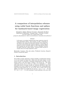
Figure 1.1 shows Alberta hourly spot price between January 01, 2011 and December 31,
2012. We can see that the prices show spikes up to $1000 per MWh and revert back to a
long run equilibrium price level. They also show a seasonal trend of low price period in the
second quarter and high prices in the third quarter.
4
H our ly Sp ot Pr ic e ( $/MW h)
1500
1000
500
0
0
1000
2000
3000
4000
5000
6000
7000
8000
9000
6000
7000
8000
9000
H ourly Sp ot Pr ic e ( $/MW h)
H our s in 2011
1500
1000
500
0
0
1000
2000
3000
4000
5000
H our s in 2012
Figure 1.1: Alberta hourly spot price in 2011 and 2012
Generally, electricity price modelling approaches can be grouped into two classes as spot
price models and forward price models.
1.2.1 Spot Price Modelling
Most of the spot price modelling approach involves at least two factors: one for capturing
the short-term hourly or daily price dynamics modelled by mean reversion and very high
volatility and the second factor representing the long term price behaviour in the forward
market. The hourly spot price dynamics can thus be captured by fitting the models to
historical spot prices.
Schwartz (2000) was the first to model the spot price accounting for the mean reversion.
Lucia and Schwartz (2000) modelled the spot price as an exponential function of the sum of
a mean reverting OU process Xt and a deterministic seasonal function f (t). The spot price
5
St can be written as
dXt = −αXt dt + σ dWt
St = exp(f (t) + Xt ),
where W is a standard Brownian motion and σ is a volatility and α is the speed of mean
reversion. But their model didn’t incorporate the spike shown in electricity prices.
To incorporate jumps, Clewlow and Strickland (2000) suggested a jump component using
a Poisson process Nt with intensity λ and a jump size of J. The model can be written as
dXt = −αXt dt + σ dWt + Jt dNt
St = exp(f (t) + Xt ).
Deng (2002) presents analytical results which are based on transform analysis described in
Duffie (2000). These models to have an upward jump followed by a downward jump, the
mean reverting speed parameter α must be extremely high.
Benth (2005) also suggested that spot prices can be modelled as a linear combination of
independent pure mean reverting jump processes
St =
n
X
(i)
wi Yt ,
(i)
dYt
(i)
(i)
= −αYt dt + σi dLt , i = 1 . . . , n,
i=1
where wi are positive weights and Lt are independent increasing c´adlag pure jump processes.
Positive prices are guaranteed in this model by allowing only positive jumps.
Another approach by Barlow (2002) modelled the demand supply equilibrium, where the
underlying electricity demand is an O-U process Xt and for some supply function u the spot
price is determined from the demand supply equilibrium equation
u(St ) = Xt ,
where u : R+ → [0, k].
Cartea and Figueroa (2005) presented a mean reverting jump diffusion model where the
deterministic seasonal function is determined by fitting the monthly historical averages with
6
a Fourier series of order 5. The paper calibrated the model parameters using the UK and
Wales historical electricity spot price data and they pointed out the difficulty of calibrating
the model to historical spot prices. The paper also noted that maximum likelihood estimation
approach employed for parameter calibration gives incorrect result.
Although the above models provide good and reliable descriptions of the dynamics of
electricity prices and are relatively simple to modify and extend, one of the shortcoming of
these models is that it is challenging and difficult to estimate parameters with a very few
market data. In addition, these models follow a parametric approach in terms of modelling
the seasonal function. Our approach, instead, estimates all the model parameters involved
based on Bayesian estimation using the historical data. A new modelling approach using
Bayesian penalized splines will be used for estimating the seasonal function.
Another approach by Liebl (2013) proposed a functional factor model that relates the
hourly electricity spot prices yth of day t with a smooth price - demand function Xt using
yth = Xt (uth ) + th ,
where uth denotes electricity demand at hour h of day t and th is assumed to be a white
noise process. The price - demand functions Xt (u) is modelled by a functional factor model
defined by
Xt (u) =
K
X
βtk fk (u),
k=1
where the factors or basis functions fk are time constant and βtk are factor scores allowed to
be nonstationary time series. First the author estimated the daily price - demand functions
ˆt by cubic spline smoothing for all days. The second step is to determine a K < ∞
X
dimensional common functional basis system f1 , . . . , fK for the estimated price - demand
ˆ1, . . . , X
ˆT .
functions X
7
1.2.2 Forward Price Modelling
Backing out forward prices from spot price based models will in general not be consistent
with market observed forward prices. As a solution to this, a lot of research has focused
on modelling the evolution of the whole forward curve. Market models for forward prices
are dated back to Black (1976) where a single forward contract is considered. Clewlow and
Strickland (1999), Koekabaker and Ollmar (2001) and Carmona and Durrleman (2003) apply
the idea of term structure modelling from Heath, Jarrow and Merton (1992) to model the
dynamics of the whole forward curve. The stochastic differential equation for the dynamics
of the forward curve with maturity T in these models is given by
n
X
dF (t, T )
= µ(t, T )dt +
σk (t, T )dWk (t),
F (t, T )
k=1
t ≤ T,
where W = (W1 , . . . , Wn ) is n-dimensional standard Brownian motion, and the drift term µ
and the n volatilities σk are deterministic functions of the current date t and maturity T .
Such models have the advantage that the market can be considered as being complete
and standard risk-neutral pricing may be used. One of the drawbacks of these models is that
forward prices do not reveal information about the price behaviour on a fine granularity of
time scale such as hourly or daily. In addition, unlike interest rate term structure models
with a fixed maturity T , electricity forward contracts have delivery periods, and market data
for fixed time delivery do not exist. As a result, these models are not directly suitable for
modelling electricity forward curves.
Fleten and Lemming (2005) presented a different approach of constructing approximated
high resolution electricity forward price curves. Average based contracts with delivery over
a period [T1 , T2 ] were considered, as in Bjerksund (2000). Let F (T1 , T2 ) be the price of the
forward contract with delivery in [T1 , T2 ] and ft be modelling constructs price of a forward
contract for fixed delivery time t within the period [T1 , T2 ] if such a contract is traded in the
8
market. Then
F (T1 , T2 ) = PT2
1
t=T1
e−rt
T2
X
e−rt f
t.
t=T1
The forward prices are constrained using the bid ask market information from the Nordic
power exchange as
F (T1 , T2 )bid ≤ PT2
T2
X
e−rt f
1
t=T1
e−rt
t
≤ F (T1 , T2 )ask .
t=T1
The seasonal variation shape of the forward curve is thus optimized using the above bid ask
information bundled with information from the forecasts generated by bottom up models.
Benth, Koekebakker and Ollmar (2007) also presented a method of estimating a smooth
forward curve from these average based contracts as, described in Section 1.1.
Borak and Weron (2008) introduced the dynamic semiparametric factor model (DFSM)
for modelling electricity forward curves. The model represents the observed forward electricity prices Yt,j using a linear combination of nonparametric loading functions ml and
parameterized common factors Zt,l as
Yt,j = m0 (Xt,j ) +
L
X
Zt,l ml (Xt,j ) + t,j ,
l=1
where Xt,j is observable covariates that represents the delivery periods. The loading functions
ml (.) is modeled with B-spline as
ml (Xj ) =
K
X
al,k ψk (Xj ),
k=1
where K is the number of knots, ψk (.) are the splines and al,k are spline coefficients. The
estimation is thus carried out by least square minimization scheme.
Fleten and Lemming (2005) and Benth, Koekebakker and Ollmar (2007) models employ
either a parametric form or a bottom up forecast for the seasonal function. Borak and
Weron (2008) approach however is heavily dependent on the number of loading functions
employed in the model. In addition, small market data poses a problem in the least square
minimization scheme.
9
Our approach however does not rely on any parametric form or forecast but provides
a method of constructing the smooth forward curve using Bayesian spline, which naturally
works well with small dataset. We also provide a method of estimating forward curves for
an illiquid hub from a liquid hub by incorporating a prior information about the hubs.
1.3 Market Description
The empirical analysis of this thesis is based on the market data from ICE quoted to Mid-C
market hub and the historical spot prices from Alberta. The following two sections give an
overview of the Alberta and Mid-Columbia markets as well as the summary of the forward
contracts traded at ICE.
1.3.1 Alberta Electricity Market
Since deregulation in 1996, Alberta electricity market operates as a wholesale power market
where the power produced and consumed as well as prices for each and every hour of the
year are facilitated and regulated by the Alberta Electric System Operator (AESO).
One of the key features of Alberta electricity spot market is that the price is highly volatile
from hour to hour. Unexpected short term outage at the power plant coupled with extreme
weather can spike the price as high as $1000/MWh for several hours. On the other hand,
surplus production together with low demand makes the price to fall as low as $0/MWh.
However, longer term prices, which can be thought of as an average of many hourly
prices, are much more stable because overall price trends tend to be driven by economical
forecasts such as demand growth, capacity additions and retirement.
Alberta has about 14,000 MW of installed electricity generation capacity as well as 21,000
kilometres of transmission lines. Together, this system continuously delivers electricity to
homes, farms and businesses in every corner of the province. About 41 percent of Alberta’s
installed electricity generation capacity is from coal and almost 40 percent from natural gas.
10
Alberta also uses water, wind, biomass and waste heat as forms of electricity generation.
We collected Alberta hourly spot prices from January 01, 2010 to December 31, 2012 to
be used for the empirical analysis in the spot price modelling approach which we present in
Chapter 5.
1.3.2 Mid-Columbia (Mid-C) and California Oregon Border (COB) Markets
The Mid Columbia (Mid-C) is a power market hub located in the state of Washington. It
serves as a common market pricing point used for trading physical and financial electricity
products through brokers in the northwest electric market, which also includes the states of
Oregon, Idaho, Utah, Nevada, Montana, Wyoming and part of California.
The region relies on hydroelectric production for approximately two thirds of its electricity
needs. The hydropower is generated from hydro dams built across the Columbia river, which
flows from the base of the Canadian Rockies in southeastern British Columbia to the states
of Washington and Oregon and flows to the Pacific ocean.
Figure 1.2: The North West Electric
Power Markets (www.ferc.gov)
Figure 1.3: Columbia River & Bonneville
dam (www.wikipedia.org). Source: U.S.
Army Corps of Engineers, 2003.
11
The volume of water in the Columbia river varies seasonally, depending on the timing
and volume of melting snowpack and precipitation. In Canada, the highest flows occur
between May and August; the lowest between December and February. In the U.S., peak
flows typically occur between April and June; the lowest also occur between December and
February.
Based on the seasonal variations of the water level through out the year, electricity
prices also show a seasonal price pattern opposite to the water level. When peak flows occur
between April and June, power prices will be generally at their lowest and in the months
between December and February they will be relatively higher.
The California Oregon Border (COB) is another pricing hub located in the state of Oregon
where the price pattern is dictated by Mid-C prices. Unlike Mid-C which is one of the most
liquid hubs in North America where power contracts are traded daily, COB is an illiquid hub
with limited market activities.
1.3.3 Inter Continental Exchange (ICE)
A market based in Atlanta, Georgia that facilitates the electronic exchange of energy commodities, ICE operates completely as an electronic exchange. It is linked directly to individuals and firms looking to trade in oil, natural gas, jet-fuel, emissions, electric power and
commodity derivatives.
ICE was established in May 2000, and has been at the forefront of the commodities
exchange market since then. The ICE network offers companies the ability to trade energy
commodities with another company around the clock and spanning the globe. ICE also
facilitates the exchange of emissions contracts and over-the-counter energy exchange.
One of the many products of ICE traded is electricity forward with delivery over a period
rather than at a fixed point in time which is the main focus of the thesis. The delivery
periods are standardized and may range from monthly to yearly contracts and they may
overlap such as yearly overlaps with quarterly and quarterly contracts overlap with monthly.
12
On the delivery period, cash settlement is based up on the mathematical average of the daily
prices calculated by averaging the peak hourly and and off peak hourly prices published by
ICE. We can think this settlement as a fixed verses float swaps where we are swapping the
monthly forward contract price (fixed price) by the daily spot price (float price).
Mid-C average based forward contracts are traded at ICE based on the time of use as
peak or off peak. Peak electricity forwards are defined based on the times of the delivery of
electricity during the peak hours defined as Monday to Saturday between hour ending 07:00
to hour ending 22:00 www.theice.com.
The market data used for empirical analysis is Mid-C forward prices traded between
December 01, 2009 - December 31, 2009 to be delivered on the peak hours between the years
2010 and 2012. The 2010 prices are monthly data, however 2011-2013 are quarterly prices
which are a single forward price for the three months of the year.
1.4 Overview of Thesis
The thesis focuses on three problems concerning the construction of electricity price curves.
The first involves the development of a Bayesian penalized spline model and associated
methodologies for the construction of a smooth forward price curve delivery at a fixed time
from average based electricity contracts delivery over a period. The proposed model is
numerically illustrated using the monthly market data quoted to Mid-Columbia pricing hub
on December 01, 2009 for delivery on January - December 2010.
The second concerns the construction of another smooth forward price curves for an
illiquid hub (COB) with limited market information by adding a spread term to the already
estimated curve for a liquid hub (Mid-C). These entail the construction of joint Bayesian
models that incorporate the positive spread between the hubs as an informative prior. It
also concerns with the evolution of these forward prices over different trading days. The
methodology is applied 22 times independently to Mid-C and COB forward prices obtained
13
from December 01 - December 31, 2009.
The third concerns the estimation of spot prices, with special attention to the construction
of daily prices from historical settled prices in the Alberta electricity market. This involves
the construction of models that flexibly represent the complex dependence structures between
seasonality, spikes and mean reverting that is exhibited in electricity spot prices. The thesis
is thus organized as follows.
Chapter 2 presents brief introduction to Bayesian estimation techniques that focuses on
Bayes formula, choice of priors and MCMC algorithm. Bayesian parametric estimation of
an O-U type spot price model and detail numerical results on the parameter estimates and
their Bayesian credible intervals are presented.
In Chapter 3, we provide a brief background introduction on smoothing spline, penalized
spline and Bayesian penalized spline that are necessary for the development of this thesis.
The chapter begins by laying out the theoretical basis of regression spline models, and it
illustrates by example the power of penalized spline models over other regression model.
MCMC algorithm and hierarchical Bayesian methodologies are also discussed in detail.
In Chapter 4, we discuss the construction of a smooth forward curve based on Bayesian
penalized spline. Our approach follows Bjerksund (2000) which models the relationship
between the forward price function at any fixed time t and the average based contracts over
the delivery period [T1 , T2 ]. Let F (t, T1 , T2 ) be the contract price of electricity at time t to
be delivered over a period [T1 , T2 ] and assuming constant cash flow throughout the delivery
period, the expression of the average based contract is
F (t, T1 , T2 ) =
Z T2
w(t, u)f (t, u) du,
T1
where
e−r(t−u)
−r(t−u) du
T1 e
w(t, u) = R T2
and f (t, u) is is the price of a forward with fixed-delivery time at u. By taking zero interest
14
rate, we can get a very good approximation to the above model as
F (t, T1 , T2 ) ≈
1
T2 − T1
Z T2
f (t, u) du.
T1
Assuming delivery occurs at a discrete delivery times, the above integral turns into a sum
and the whole expression will turn into an average of f (t, u) over the delivery periods which
we use for our numerical computation.
The forward curve f inside the above integral is modelled as a spline the same way as Li
and Yu (2005) and we estimate the smoothing parameter from the ratio of variances of the
posterior distribution inside the MCMC algorithm employed. The chapter also presents a
way of extending the smooth forward curve to a long term price curve beyond the one year.
A two step construction methodology from Bayesian perspective is also presented in
Chapter 4. The Mid-Columbia smooth forward curve is first estimated with a Bayesian
penalized spline model. The California Oregon Border curve is then constructed by adding
a spread to the already estimated Mid-C curve. The positive spread between Mid-C and
COB is incorporated as an informative prior. Finally, the methodology is illustrated using
the market data from Mid-C and few COB monthly forward prices and results from the
simulation study is summarized and the fitted surfaces are presented.
Motivated by the ease of parameter estimation of a spot price model using Bayesian
paradigm, we present spot price modelling approach using a Bayesian penalized spline
smoothing in Chapter 5. Our approach follows Lucia and Schwartz (2002) spot price modelling approach but we apply penalized spline smoothing to the monthly average of historical
spot prices to estimate the deterministic seasonal function f . After removing the seasonal
function from the log of the historical spot price, we left with a pure stochastic O-U process
for which we can estimates the parameters using Bayesian and MCMC algorithm. Using the
estimated parameters and the seasonal function, spot prices are constructed back to see how
the model fits the observed prices. Mathematical formulations, graphical representations
and numerical results are presented in detail.
15
Finally, in Chapter 6, results from the thesis are summarized, issues associated with
spline modelling are discussed, and recommendations are presented regarding the methods
considered throughout the thesis. Potential areas for future research are pointed out as well.
16
Chapter 2
Bayesian Estimation of Spot Price Model
2.1 Introduction
Electricity spot and forward price models are mostly stochastic in nature and are governed
by a set of continuous-time stochastic differential equations. While this modelling approach
is very common in theoretical analysis, numerical estimation of model parameters is difficult
and poses serious challenges.
The natural choice for empirical estimation of model parameters is to use a maximum
likelihood estimation (MLE) approach. However in most cases the likelihood function is
unknown or has a nonstandard form which makes the implementation difficult. One approach
is to employ an approximate likelihood function but it induces bias in parameters values as
noted in Gray (2005).
In addition, MLE is based on the assumption of large number of samples, and as a result
the approach may produce incorrect estimates under a limited number of samples case. This
is the case pointed out by Cartea and Figueora (2005) who applied MLE on UK and Wales
electricity markets. They found out that the MLE approach produces negative values for
parameters that should otherwise be positive.
In order to avoid these difficulties posed in parameter estimation, we propose Bayesian
approach as a natural solution. The Bayesian paradigm makes use of a prior information
about the parameters and models the joint posterior distribution conditioning on the given
data using Bayes’ formula. Estimation of the parameters is performed using a Markov Chain
Monte Carlo algorithm based on Gibbs sampling and Metropolis Hastings algorithm.
In this chapter, we examine the Bayesian estimation approach to estimate parameters of
a continuous time O-U spot price model where the mean reversion parameters do not have
17
a standard density. An MCMC scheme based on Gibbs sampling for the long run mean and
volatility parameters and Metropolis Hastings algorithm for the mean reversion is employed.
The estimates for the parameters are then compared against results from the maximum
likelihood estimation.
The remainder of the chapter is organized as follows. Section 2.2 presents a brief overview
of Bayesian estimation framework. Section 2.3 provides noninformative and conjugate priors.
MCMC algorithms together with Gibbs and Metropolis Hastings steps are presented in
Section 2.4. The continuous time O-U spot price model together with MLE and Bayesian
estimation of the parameter are discussed in Section 2.5. Section 2.6 illustrates the Bayesian
methodology applied to a simulated samples from the proposed model and numerical results
are presented and summarized in a table.
2.2 Bayesian Estimation Technique
Bayesian statistical inferences about the parameter θ are made conditional on the observed
data and takes the parameters as random variables. Suppose that θ has a probability
distribution p(θ). Then from Bayes theorem we have
p(Y |θ)p(θ) = p(Y, θ) = p(θ|Y )p(Y ).
Conditional on the observed data Y , the distribution of θ is
p(θ|Y ) =
p(Y |θ)p(θ)
.
p(Y )
Given the data Y , the p.d.f. p(Y |θ) may be regarded as a function of θ, which we recall as
the likelihood function of θ given Y and written as L(θ|Y ). So, given a likelihood L(θ|Y )
and a prior probability density p(θ), the posterior density for θ is given as
p(θ|Y ) =
p(θ)L(θ|Y )
.
p(Y )
18
The factor p(Y ) does not depend on θ and, can thus be considered a constant, yielding
p(θ|Y ) ∝ p(θ)L(θ|Y ).
This expression condenses the technical core of the Bayesian estimation technique: the primary task of any estimation is to develop the model p(θ, Y ) and perform the necessary
computation to summarize p(θ|Y ). In most cases, analytic evaluation of the estimates
θˆ = E[θ|Y ] is impossible so that alternative approaches such as Markov Chain Monte Carlo
(MCMC) can be used. Moreover, specification of the prior p(θ) is also a challenge so that
noninformative and conjugate priors are considered.
2.3 Specification of Prior
The prior distribution represents a subjective information or an expression of belief about
an unknown quantity before the data are available. Generally, there are two classes of prior
distributions: noninformative priors and conjugate (informative) priors.
2.3.1 Noninformative Priors
In cases where we do not have a strong prior belief or lack of information about the parameter, it is advisable to use noninformative prior which is dominated by the likelihood function
as in Tanner (1996). We considered two cases to illustrates the choice of noninformative
priors.
Case 1: Normal population (mean unknown, variance known).
Consider an iid sample from a N (θ, σ 2 ) population, where σ 2 is known and θ is unknown.
Note that the likelihood function f (Y |θ) is equal to
n
Y
®
1
1 (yi − θ)2
exp
−
2
2
σ2
i=1 2πσ
´
n
1
1X
(yi − θ)2
=
exp
−
.
(2πσ 2 )n/2
2 i=1
σ2
(
19
)
Since σ 2 is given, (2πσ 2 )−n/2 is considered a constant and does not help to determine the
shape of the likelihood hence can be omitted. We also note that
n
X
(yi − θ)2 =
i=1
since
Pn
i=1 (yi
n
X
[(yi − y¯) + (¯
y − θ)2 =
i=1
n
X
(yi − y¯)2 + n(¯
y − θ)2 ,
i=1
− y¯)(¯
y − θ) = 0. Thus, the likelihood can be re-expressed as
®
1
exp −
2
Pn
i=1 (yi
´
− y¯)2 + n(¯
y − θ)2
.
σ2
Conditional on the data,
−
n
1X
(yi − y¯)2
2 i=1
σ2
is a constant. Hence, we have the further reduction that the likelihood can be expressed as
®
´
y − θ)2
1 n(¯
exp −
.
2
σ2
Under the prior p(θ) ∝ constant, it follows that the posterior density is N (¯
y , σ 2 /n). Under
the prior p(θ) = N (θ0 , σ02 ), where θ0 and σ0 are known constants, it can be shown that the
posterior density is normal with mean given by a weighted average of the prior mean and
the sample average:
Ç
θ0
1/σ02
1/σ02 + n/σ 2
å
Ç
å
n/σ 2
+ y¯
,
1/σ02 + n/σ 2
and the posterior variance is equal to (1/σ02 + n/σ 2 )−1 . Note that as σ0 → ∞ (n is fixed)
or as n → ∞ (σ0 fixed) the prior flattens out and we recover the posterior under the prior
p(θ) ∝ constant discussed in Gelman (1995) and Tanner (1996).
In general, if we can write the likelihood L(θ|Y ) in the form g[ψ(θ) − t(Y )], then the
likelihood is in data-translated form, since different datasets only shift the likelihood through
t(Y ) as discussed in Tanner (1996). So we can take p(ψ(θ)) ∝ constant, since it is on the
ψ(θ) scale that the likelihood is data-translated thus, a noninformative prior would say
that any value is reasonable on the ψ(θ) scale. Transforming back to the θ scale, we have
p(θ) ∝ | ∂ψ(θ)
|.
∂θ
20
Case 2: Normal population (mean known, variance unknown)
Let y1 , · · · , yn be an iid sample from N (µ, σ 2 ), then L(σ|Y ) = σ −n exp
s2 =
Pn
i=1 (yi
Ä
−ns2
2σ 2
ä
, where
− θ)2 /n. Now note that
Ç
σ −n
−ns2
exp
s−n
2σ 2
å
ï
Å ãò
ñ
Ç
Ç
ååô
−n
s2
× exp
exp log
2
σ2
n
= exp(−n(log σ − log s) − exp[−2(log σ − log s)]).
2
σ
= exp −n log
s
In this case, g(y) = exp(−ny −
n
2
exp(−2y)), t(Y ) = log s and ψ(θ) = log σ. Hence, arguing
as above we would put a flat prior on log σ, i.e. p(log σ) ∝ constant, which implies that
p(σ) ∝ σ1 .
When both θ and σ are unknown, we argue that knowledge of θ should be independent
of σ and vice versa. Thus, p(θ, σ) = p(θ)p(σ 2 ) ∝ constant × σ12 ∝
1
σ2
as presented in Gelman
(1995) and Tanner (1996).
2.3.2 Conjugate Priors
In some situations, the data analyst may not wish to be vague and may be willing to use
some smooth distribution that is a specific member of a family of distributions. One such
class of distributions is the conjugate class.
If the likelihood is based on a random sample of size n from an exponential family
distribution with density

m
X
g(θ)h(y) exp 
j=1


φj (θ)tj (y) ,
then a conjugate prior density of the form

m
X
p(θ) ∝ [g(θ)]b exp 
j=1


φj (θ)aj 
combines with the likelihood to yield a posterior density having the same form as the prior
density, but with b, a1 , · · · , am replaced by
b0 = b + n, a0j = aj +
m
X
i=1
21
tj (y), j = 1, · · · , m.
It can be seen that the gamma distribution is conjugate to the Poisson, the normal distribution is conjugate to the normal (with known σ and unknown µ), and the inverse gamma
(IG)1 is conjugate to the normal (unknown σ and known µ).
2.4 Markov Chain Monte Carlo (MCMC)
MCMC is an estimation approach which provides an efficient estimates to the parameter
of interest asymptotically. It also provides the finite sample distribution. The sampling
based MCMC method avoids the computation of a high-dimensional integral necessary for
obtaining the marginal distribution of parameters. Instead, it generates random samples
from any nonstandard likelihood functions. These random samples converge to finite sample
distribution of the estimates.
MCMC methods have been mostly applied in Bayesian applications where probability
densities are known up to a constant of proportionality. The interest of estimation is on the
posterior marginal distribution p(θ|Y ) and the point estimate θˆ = E[θ|Y ]. Computing the
expectation involves integration and is often analytically difficult as θ is high dimensional.
MCMC method thus generates random samples of observations from p(θ|Y ) namely {θ n :
n = 1, . . . , N } and provides a density estimator that converges in distribution to the marginal
density p(θ|Y ). Thus, posterior mean and standard deviation of parameter θ can thus be
evaluated using
θˆ =
‘
Var(θ|Y
)
1
N
1 X
θn
N n=1
(2.1)
N T
1 X
=
θ n − θˆ θ n − θˆ .
N − 1 n=1
θ ∼ Inverse-gamma(α, β), if the p.d.f of θ is p(θ) =
22
β α −(α+1) −β/θ
e
,
Γ(α) θ
α > 0, β > 0 and θ > 0.
(2.2)
2.4.1 Gibbs Sampling Technique
Gibbs sampling is an MCMC sampling-based approach used for estimating marginal density.
Gibbs sampler has been applied in the context of stochastic models involving large numbers
of variables. Gelfand and Smith (1990) employed the technique in a variety of models,
including multinomial, multivariate normal, hierarchical and k groups mean models.
Assume the distribution of interest be π(θ), where θ = (θ1 , . . . , θd )0 and the full conditional distributions πi (θi ) = π(θi |θ−i ), i = 1, . . . , d are completely known and can be sampled
from. Here θ−i = (θ1 , θ2 , . . . , θi−1 , θi+1 , . . . , θd ) is the vector θ with its ith component removed. The interest is to draw samples from π when direct sampling scheme is not available
but drawing from πi is possible. Gibbs sampling provides a way of sampling successive draws
from the full conditional posterior distributions. The steps in the algorithm are
(0) 0
(0)
1. Set initial values θ(0) = θ1 , . . . , θd
.
(j) 0
(j)
2. Obtain a new value θ(j) = θ1 , . . . , θd
(j−1)
from θd
through successive gen-
eration of values
(j)
(j−1)
, . . . , θd
(j)
(j)
(j−1)
(j−1)
(j)
θ1 ) ∼ π θ1 |θ2
(j−1)
θ2 ) ∼ π θ2 |θ1 , θ3
, . . . , θd
,
,
..
.
(j)
(j)
θd ) ∼ π θd |θ1 , . . . , θd−1 .
3. Update j = j + 1 and repeat step 2 until convergence is achieved.
When convergence is reached, the resulting value θ(j) is a draw from π.
2.4.2 Metropolis Hastings Algorithm
Metropolis algorithm is another MCMC algorithm required when one or more of the full
conditionals are not available in closed form but the functional form of joint density p(θ|Y ) =
23
p(θ1 , . . . , θd |Y ) is known. Gibbs sampler cannot be applied to situations where conditional
densities are unavailable or not easy to sample directly from.
The Metropolis algorithm was first developed in Metropolis (1953). It can be used to
generate random samples from any target distribution known up to a normalizing constant,
regardless of its analytical complexity and its dimensionality.
The interest is to generate random samples that have a stationary distribution π. One of
the contributions of Metropolis algorithm is in constructing the transition density p(θ, φ) that
realizes a Markov chain with equilibrium distribution π. It is equivalent to find transition
matrix P that realizes a reversible chain, which satisfies π = πP . That is, for all i 6=
j, πi pij = πj pji . In other word, p(θ, φ) must be a reversible chain and satisfy the detailed
balance equation
π(θ)p(θ, φ) = π(φ)p(φ, θ).
The proposed state φ is generated from a symmetric proposal transition density that
satisfies q(θ, φ) = q(φ, θ). The new state is thus accepted with a probability α(θ, φ) given by
®
´
π(φ)
α(θ, φ) = min 1,
,
π(θ)
and the new state is rejected with probability 1 − α(θ, φ).
The algorithm was further generalized to an arbitrary transition density in Hastings
(1970). The proposal density q(θ, φ) does not have to be symmetric. The proposed state φ
in this case is accepted with probability α(θ, φ) given by
®
´
π(φ)q(φ, θ)
.
α(θ, φ) = min 1,
π(θ)q(θ, φ)
There are other acceptance probability specifications that generate reversible chains, such
as in Barker (1965). Peskun (1973) concludes that the Metropolis acceptance-rejection rule
is optimal in the sense of having the smallest asymptotic variance for the resulting estimates.
By the standard Markov chain theory, if the chain is irreducible, aperiodic and reversible,
24
it will converge to its equilibrium distribution π(x), which is the case with the Metropolis
algorithm. Moreover, after a sufficient burn-in steps, the samples produced from the chain
can be used to approximate the target distribution.
The closeness of the proposal density to the the target distribution is one of the factors
which determine the efficiency of Metropolis Hastings sampler. Common candidate proposal
densities are multivariate normal density and multivariate t distribution. Theoretically, the
proposal density in MH algorithm is not required to have any good global properties and
can take any form in Hastings (1973) generalization.
The steps in Metropolis Hastings algorithm can be summarized as below.
1. Initialize the iteration counter of the chain j = 1 and set initial values θ (0) .
2. Move the chain to a new value φ generated from the density q(θ (j−1) , ·).
3. Evaluate the acceptance probability of the move α(θ (j−1) , φ) given by
®
´
π(φ)q(φ, θ)
.
α(θ, φ) = min 1,
π(θ)q(θ, φ)
4. Generate an independent uniform quantity u and
• If u ≤ α then the move is accepted and θ (j) = φ.
• If u > α then the move is rejected and θ (j) = θ(j−1) .
5. Change the counter from j to j + 1 and return to step 2 until convergence is
reached.
The capability of MCMC algorithms to work with high dimensions leads to many applications in Finance. Aguilar and West (2000) use MCMC and sequential filter to estimate
dynamic factor models, with international exchange rates data. The applications on termstructure models are mostly with stochastic volatility models. Jaquier, Polson & Rossi (1994)
shows that the Bayesian Markov chain estimators outperform estimators from moment and
QML methods on stochastic volatility models.
25
2.5 O-U Spot Price Model
The O-U process is the unique solution to the following stochastic differential equation
dXt = θ(µ − Xt )dt + σdWt , X0 = x0 ,
where σ is interpreted as the volatility or diffusion, µ is the long-run mean (equilibrium)
value of the process, and θ is the speed of reversion.
Using the Itˆo lemma with f (t, x) = xet , one can show the explicit solution of the above
SDE as
−θt
Xt = µ + (x0 − µ)e
The random variable It =
R t −θ(t−u)
e
dW
u
0
+σ
Z t
0
e−θ(t−u) dWu .
appearing on the right-hand side of the above
equation is normally distributed with mean zero and variance
Z t
1
(1 − e−2θt ).
2θ
e−2(t−u) du =
0
Thus, Xt is normally distributed with mean µ + (x0 − µ) e−t and variance
Ç
σ2
(1
2θ
− e−2θt ).
å
Xt ∼ N µ + (x0 − µ)e
−θt
,
σ2
(1 − e−2θt ) .
2θ
2.5.1 Maximum Likelihood Estimation (MLE)
A maximum likelihood estimate (MLE) of θ is a value of θ that maximizes the likelihood
L(θ|Y ) or, equivalently, the loglikelihood l(θ|Y ).
ˆ is unique, θˆ is the value of θ
In situations where the maximum likelihood estimate (θ)
best supported by the data. Alternatively, θˆ is the value of θ which makes the observed
value of the data most likely. It is noted that if g(θ) is a 1-1 function of θ and θˆ is an MLE
ˆ is an MLE of g(θ). This is called the invariance property of MLE.
of θ, then g(θ)
Suppose the likelihood is differentiable, unimodal, bounded above, and θ is of dimension
d. Then the mode θˆ is obtained by
26
0.8
0.6
3.0
P(t,x)
2.5
0.4
2.0
0.0
Tim
e
0.2
1.5
-3
1.0
-2
-1
0
x
1
0.5
2
3
Figure 2.1: Transition density of the O-U process starting at x0 = 0 with µ = 0, θ = 1, σ 2 = 2
1. Differentiating the loglikelihood with respect to θ to obtain the d × 1 vector
∂l(θ|Y )/∂θ.
2. Setting the d dimensional likelihood equations to 0, i.e. ∂l(θ|Y ) = 0.
3. Solving for θ.
When the loglikelihood is quadratic, the likelihood equations are linear in θ and the
solution is relatively easy to obtain. In more general situations where a closed-form solution
of the likelihood equations cannot be found, one may use an iterative numerical method to
locate a mode as in Tanner (1996).
27
2.5.2 MLE of the O-U Model
Assume a discrete sample of size n + 1 at equally spaced intervals h, X = (X0 , Xh , . . . , Xnh ).
The O-U process has a normal transition density
Ç
p(Xjh |X(j−1)h ) =
å− 21
πσ 2
(1 − e−2θh )
θ
θ(Xjh − X(j−1)h e−θh − µ(1 − e−θh ))2
exp −
.
σ 2 (1 − e−2θh )
"
#
The likelihood function L(θ, µ, σ 2 |X) is given by
L(θ, µ, σ 2 |X) =
n
Y
p(Xjh |X(j−1)h )
j=1
Ç
=
å− n2
πσ 2
(1 − e−2θh )
θ

θ

exp 
−
n
P
[Xjh − X(j−1)h e−θh − µ(1 − e−θh )]2
j=1
σ 2 (1
−
e−2θh )


.

The log-likelihood function l(θ, µ, σ 2 |X) = log(L(θ, µ, σ 2 |X)) can be derived from the above
conditional density function as
l(θ, µ, σ 2 |X) =
n
X
j=1
ln p(Xjh |X(j−1)h )
Ç
å
n
n
σ2
= − ln(π) − ln
(1 − e−2θh )
2
2
θ
n
X
θ
−
[Xjh − X(j−1)h e−θh − µ(1 − e−θh )]2 .
σ 2 (1 − e−2θh ) j=1
The maximum likelihood estimates (MLE) of the parameters can be found by taking the
partial derivative of the log-likelihood function and set it to zero and solving the equation
28
as follows.
∂l(θ, µ, σ 2 |X)
= 0
∂µ
=
n
X
θ
2[Xjh − X(j−1)h e−θh − µ(1 − e−θh )](1 − e−θh )
σ 2 (1 − e−2θh ) j=1
n
P
⇒ µMLE =
[Xjh − X(j−1)h e−θh ]
j=1
n(1 − e−θh )
∂l(θ, µ, σ 2 |X)
= 0
∂σ 2
n
X
n
θ
= − 2+ 4
[Xjh − X(j−1)h e−θh − µ(1 − e−θh )]2
−2θh
2σ
σ (1 − e
) j=1
2
⇒ σMLE
=
n
X
2θ
[Xjh − X(j−1)h e−θh − µ(1 − e−θh )]2
−2θh
n(1 − e
) j=1
∂l(θ, µ, σ 2 |X)
= 0
∂θ
=
n
2θhe−θh X
[(Xjh − µ)(X(j−1)h − µ) − e−θh (X(j−1)h − µ)2 ]
σ 2 (1 − e−2θh ) j=1
n
P
⇒ θMLE
(X − µ)(X(j−1)h − µ)
1 j=1 jh
= − ln
.
n
P
h
(X(j−1)h − µ)2
j=1
2.5.3 Bayesian Estimation of the O-U Process
Bayesian estimation technique is a widely used technique in finance and there are many
valuable contributions of the Bayesian approach to research. For example, Gray (2002) has
studied the Vasicek interest rate model using the Bayesian approach.
Assume a discrete sample of n + 1 interest rates at equally spaced intervals h, X =
(X0 , Xh , . . . , Xnh ). The O-U interest rate has a normal transition density
Ç
p(Xjh |X(j−1)h ) =
å− 21
πσ 2
(1 − e−2θh )
θ
θ(Xjh − X(j−1)h e−θh − µ(1 − e−θh ))2
.
exp −
σ 2 (1 − e−2θh )
"
29
#
The likelihood function L(θ, µ, σ 2 |X) is given by
2
L(θ, µ, σ |X) =
n
Y
p(Xjh |X(j−1)h )
j=1
Ç
=

å− n2
2
πσ
(1 − e−2θh )
θ
1
,
σ2
Assuming a flat prior p(σ 2 ) ∝
θ

exp 
−
n
P
[Xjh − X(j−1)h e−θh − µ(1 − e−θh )]2
j=1


.

σ 2 (1 − e−2θh )
which corresponds to IG(0,0), and the fact that the
inverse gamma (IG) is conjugate prior to the normal (unknown σ and known µ), we have
the conditional density
Ñ
p(σ 2 |X, µ, θ) ∼ IG
Ç
å
n
X
n
θ
,
[Xjh − X(j−1)h e−θh − µ(1 − e−θh )]2
2 1 − e−2θh j=1
é
.
Moreover, the normal distribution is conjugate prior to the normal (with known σ and
unknown µ), and we have the conditional density
Ñ
p(µ|X, σ 2 , θ) ∼ N
n
Xjh − X(j−1)h e−θh σ 2 (1 − e−2θh )
1X
,
n j=1
1 − e−θh
2θn(1 − e−θh )2
é
.
However, the conditional density of θ is non-standard. So assuming a flat prior on θ in
combination with the likelihood L(θ|X), we can use the normal based inference approach as
described below to get the candidate density for θ.
Normal-based inference
Let θˆ be the mode of the likelihood for the data set Y . Then in certain situations
ˆ ∼ N (0, C),
(θ − θ)
(2.3)
ˆ
where C is the d × d variance-covariance matrix of (θ − θ).
In Bayesian paradigm, θˆ is fixed (conditional on the data Y ) and θ is considered as
random. Given the model and the data, (2.3) indicates that the posterior density of θ is
ˆ C).
normal with mean θˆ and variance-covariance matrix C, i.e. p(θ|Y ) = N (θ,
The Bayesian justification of (2.3) is an expansion of the loglikelihood about the fixed
value θˆ (conditional on Y ),
ˆ ) + (θ − θ)
ˆ T S(θ|Y
ˆ ) − 1 (θ − θ)
ˆ T J(θ|Y
ˆ )(θ − θ)
ˆ + r(θ|Y ),
l(θ|Y ) = l(θ|Y
2
30
ˆ ) = −∂ 2 l(θ|Y )∂θ2 | ˆ and J(θ|Y ) is called the observed information matrix. Since
where J(θ|Y
θ
ˆ ) = 0, assuming that r(θ|Y ) can be neglected, then
S(θ|Y
1
ˆ T J(θ|Y
ˆ )(θ − θ)},
ˆ
L(θ|Y ) = exp(l(θ|Y )) ∼ exp{− (θ − θ)
2
which implies that the likelihood/posterior density is proportional to the multivariate normal
ˆ ) as described in Tanner
density with mean θˆ and variance-covariance matrix C = J −1 (θ|Y
(1996).
Based on the above description, we can assume that the candidate density of θ is given
by
ˆΣ ,
p(θ|X, µ, σ 2 ) ∼ N θ,
where
n
P
(X − µ)(X(j−1)h − µ)
1 j=1 jh
ˆ
θ = θM LE = − ln
,
n
P
h
(X(j−1)h − µ)2
ñ
j=1
2
2
∂ log L(θ, µ, σ |Y )
−
∂θ2
Σ =
ô−1
=
θˆ
B2
,
A0 BC − AB 0 C + ABC 0
where
A = he−θh
B =
C =
σ 2 (1 − e−2θh )
2θ
n
X
[(Xjh − µ)(X(j−1)h − µ) − e−θh (X(j−1)h − µ)2 ]
j=1
0
A
= −θhe−θh
B0 =
σ2
[(1 + 2hθ)e−2hθ − 1]
2θ2
C 0 = he−θh
n
X
(X(j−1)h − µ)2 .
j=1
So using the above candidate density and applying Metropolis Hastings method, we can
draw iterates for θ.
31
2.6 Statistical Inferences
Statistical inference of the model can then be conducted on the basis of a simulated samples
of observations from p(θ|Y ) namely {θ n : n = 1, . . . N }. The Bayesian estimate of θ as well
as the numerical standard error estimates can be obtained from
θˆ =
‘
Var(θ|Y
)
N
1 X
θn
N n=1
N T
1 X
=
θ n − θˆ θ n − θˆ .
N − 1 n=1
(2.4)
(2.5)
It can be shown that θˆ tends to E(θ|Y ) as N tends to infinity. Other statistical inference on
θ can be carried out based on the simulated sample, {θ n : n = 1, . . . N }. For instance, the
2.5% and 97.5% points of the sampled distribution of an individual parameter give a 95%
posterior interval.
As the posterior distribution of θ given Y describes the distributional behaviour of θ
with the given data, the dispersion of θ can be analyzed through Var(θ|Y ), with an estimate
given by (2.4) based on the sample covariance matrix of the simulated observations. The
‘
positive square root of of the diagonal element in Var(θ|Y
) is commonly taken as a standard
error estimate of the Bayesian estimates.
2.6.1 Numerical Example
In this example, a sequence of monthly interest rates is simulated according to the O-U
model with X0 = 0.10, θ = 0.18, µ = 0.08, and σ = 0.02 as shown in Figure 2.2. Bayesian
estimates with conjugate prior distributions are first sampled. Using the Gibbs sampling
technique, we draw σ 2 from an inverted-gamma and µ from a normal and the samples are
accepted with probability one. However, we use the Metropolis Hastings algorithm to draw
θ from the candidate normal density and the sample is accepted with some probability. As a
result, a sequence of iterates for (σ 2 , θ, µ) is generated and, after an initial warm up period,
32
0.10
0.00
0.05
Xt
0.15
Vasciek Interest Rate Path
0
100
200
300
t
Figure 2.2: O-U sample path with X0 = 0.10, θ = 0.18, µ = 0.08, and σ = 0.02
these draws converge to draws from the true, but unknown, joint distribution of parameters.
The output from the chain is used to derive point estimates of the parameters, as well as
the numerical density of any function of these parameters as in Gray (2002).
In this example, 5000 Bayesian estimates are used for each of the parameters and 2500
post warm up samples (after burn in samples) are considered. Then, the Bayesian estimates
along with maximum likelihood estimates and their numerical standard errors estimates are
obtained via (2.4) and (2.5). The results are presented in Table 2.1.
Table 2.1 shows that the standard errors computed from the simulated observations
are relatively small for the Bayesian estimates. For large sample size of 500, the Bayesian
posterior interval for the mean reverting parameter θ is tighter comparing to the Maximum
Likelihood approach. However, for the other two parameters µ & σ both approaches result
in almost the same results because their posterior distributions have standard forms. So
in case of nonstandard posterior distribution, Bayesian approach gives a tighter posterior
interval and better estimate for the parameters.
33
ML estimates
n
µ
0.076
0.023
(0.060,0.097)
5%
σ
Bayesian estimates
θ
µ
σ
θ
100
Mean
Std Err
95% Ints
Bias
0.023
0.248
0.003
0.082
(0.016,0.026) (0.081,0.369)
15%
37.7%
0.074
0.021
(0.060,0.096)
7.5%
0.023
0.003
(0.017,0.027)
15%
0.223
0.063
(0.098,0.336)
23.9%
300
Mean
0.082
0.021
0.212
Std Err
0.006
0.002
0.060
95% Ints (0.0793,0.0809) (0.018,0.024) (0.145,0.300)
Bias
2.5%
5%
17.8%
0.084
0.007
(0.075,0.094)
5%
0.022
0.001
(0.018,0.025)
10%
0.191
0.046
(0.130,0.299)
6%
500
Mean
0.081
0.021
0.194
Std Err
0.005
0.001
0.050
95% Ints (0.0796,0.0803) (0.019,0.021) (0.151,0.233)
Bias
1.3%
5%
7.8%
0.082
0.021
0.005
0.001
(0.0797,0.091) (0.019,0.021)
2.5%
5%
0.185
0.034
(0.154,0.212)
2.8%
Table 2.1: Point estimates of the O-U interest rate model
2.7 Conclusion
Spot and forward price models often use continuous time stochastic equations to model
power price dynamics. Numerical estimation of these models, however, is bottlenecked by a
variety of problems. The scarcity of historical data coupled with the complex or nonstandard
nature of the likelihood function makes the regular MLE estimation approach unfeasible. An
alternative to this will be to adopt a Bayesian approach.
The advantage of Bayesian framework is the capability of incorporating prior information
about the parameters and the ease to work with small number of sample data. Unlike
most frequentist approaches that provide point estimates, the Bayesian approach provides a
distribution for the parameters from which we can draw any kind of statistical inference.
In this chapter, we discussed a Bayesian parameter estimation of a continuous time O-U
spot price model using MCMC scheme. The long run mean µ and the diffusion parameters
σ in the model have a standard distribution, so Gibbs sampling is used to draw samples.
However, the mean reversion has unknown density and Metropolis Hastings algorithms were
applied.
34
The O-U model we illustrated has a normal transition density and an exponential type
likelihood function. In cases like this, the Bayesian and MLE approaches may give the same
result though Bayesian outperforms MLE on the estimation of the mean reversion parameter
θ.
35
Chapter 3
Bayesian Penalized Spline Smoothing
3.1 Introduction
Regression spline smoothing techniques are among some of the most widely used smoothing
methods in finance. A lot of research has been done in terms of interest rate term structure
estimation. McCulloch (1971, 1975), Vasicek and Fong (1982), Shea (1984, 1985) estimate
the discount function with regression splines. Chambers, Carleton, and Waldman (1984)
estimate the yield curve with polynomials. Adams and van Deventer (1994) estimate the
term structure using smoothing splines, applying the maximum smoothness criteria.
After the initial work by Eliers and Marx (1996), the penalized spline smoothing approach
become more popular in theoretical statistics and has recently been applied to financial
models. The underlying principle of penalized spline smoothing is to estimate an unknown
smooth function by replacing the function with a high dimensional basis representation and
impose a penality on the spline coefficient to achieve a smooth fit.
Ruppert, Wand, and Carroll (2003) linked the idea of penalized spline smoothing to linear mixed models and showed the practical application to perform any regression analysis.
Recently, Jarrow, Ruppert, and Yu (2004) estimate the term structure of US government
Treasury bond with a nonparametric penalized spline model by minimizing the sum of least
square criterion and a roughness penalty term. They also adopt a semi-parametric model
to estimate the corporate debt term structure by adding a constant credit spread to the
Treasury term.
Financial application of penalized spline smoothing modelling approaches are mostly
applied to estimating the term structure of interest rates. In terms of modelling the term
36
structure of energy forward prices using spline smoothing, not much work has been done
so far. Benth, Koekebakker and Ollmar (2007) construct a smooth curve from observed
Nord Pool electricity forward prices with settlement over a period using a polynomial spline
with a maximum smoothness property, so that the newly constructed smooth forward curve
matches the observed market prices.
Li and Yu (2005) employed the Bayesian approach to estimate the interest rate term
structure of Treasury and corporate debt as in Jarrow, Ruppert, and Yu (2004). Bayesian
penalized spline is a class of penalized spline smoothing which treats the spline coefficients as
random and assigns prior densities to characterize prior information about parameter values
before estimation. The posterior distribution of the parameters given the data is thus used
for statistical inference. The authors found out that unlike the frequentist approach the
small size of the corporate debt poses no particular difficulty.
Most of the spline smoothing and regression modelling approaches are used for interest
rate term structure modelling. Motivated by the work of Li and Yu (2005) and Benth,
Koekebakker and Ollmar (2007), we employ a Bayesian penalized spline smoothing approach
to extract a smooth forward curve from average based power contracts and to model the
seasonal function in spot price models.
In this chapter, we summarize and provide background information on smoothing and
regression penalized splines. As our estimation of the electricity price curves in the next
two chapters depend on Bayesian penalized spline, we present a brief introduction of these
smoothing spline approaches in a Bayesian framework and the numerical algorithm employed
using Markov Chain Monte Carlo (MCMC).
This chapter is organized as follows. Section 3.2 gives a brief definition of parametric
and nonparametric regression. Smoothing and regression penalized spline are discussed
and summarized in Section 3.3. Section 3.4 illustrates the different regression techniques
using example from Strontium isotopes ratio data. Bayesian penalized spline smoothing
37
and MCMC algorithm are also presented in the later Section 3.5. For additional details
on smoothing spline regression we recommend Wahba (1978, 1990), Green and Silverman
(1994), Hastie and Tibshirani (1990), Eliers and Marx (1996), Ruppert and Caroll (1997,
2002), Eubank (1999), Ruppert, Wand and Caroll (2003) and Jarrow, Ruppert, and Yu
(2004).
3.2 Parametric and Nonparametric Regression
Regression analysis builds mathematical models that estimate the functional relationship of
a dependent variable to one or more independent variables. These models may be used to
predict responses at unobserved and/or future values of the independent variables. In the
simple case when both the dependent variable y and the independent variable x are scalar
given bivariate observations (xi , yi ) for i = 1, . . . , n, a regression model relates dependent
and independent variables as follows:
yi = f (xi ) + i ,
i = 1, . . . , n,
(3.1)
where f is an unknown regression function that we wish to estimate and i ∼ N (0, σ 2 ) are
zero-mean identical independent random errors with a common variance σ 2 . We can also
write the above regression model as
yi ∼ N (f (xi ), σ 2 ).
The goal of regression analysis is to construct a model for f and estimate it based on
noisy data. Both parametric and nonparametric techniques are commonly used to find the
regression function f . A common approach is to approximate f by polynomial of order m
f (x) = β0 + β1 x + β2 x2 + . . . + βm xm .
(3.2)
The above polynomial regression is a familiar type of parametric regression and it assumes
that the form of f is known except for finitely many unknown parameters. This assumptions
38
is too restrictive and the approximations may be too crude for some applications, in particular
fitting wiggly curves like power price curves.
A nonparametric regression model does not assume a predetermined form. Instead, it
makes assumptions on qualitative properties of f . The basic idea of nonparametric regression
is to depend on the data and decide which function fits the best without imposing any specific
form on f . So it is more flexible and can uncover structure in the data that might otherwise
be missed.
Smoothing and regression penalized splines are examples of nonparametric regression and
they are a powerful and versatile tool for building models to exploit structure in data. The
idea of these penalized spline is to estimate a smooth f using a spline (basis functions) by
choosing the number and locations of knots for the spline and to introduce a penalty to
prevent overfitting. In the next sections, we provide a brief introduction about penalized
splines and Bayesian penalized splines which are a focus of this thesis.
3.3 Smoothing and Regression Penalized Spline
3.3.1 Smoothing Spline
Given data y = [y1 , . . . , yn ]T = [y(x1 ), . . . , y(xn )]T with a < x1 , . . . , xn < b and consider the
regression model (3.1)
yi = f (xi ) + i ,
i = 1, . . . , n.
The penalized sum of squares S(f ) is defined as
S(f ) = n−1
n
X
(yi − f (xi ))2 + λ
i=1
Z b
{f (m) (x)}2 dx,
(3.3)
a
where f is assumed to be a 2m − 1 differentiable function on the interval [a,b].
A smoothing spline fˆ is defined as the minimizer over twice differentiable functions f of
the penalized sum of squares:
fˆ = arg min S(f ).
39
The integral term above is considered as a roughness penalty and λ > 0 is a smoothing
parameter which governs the tradeoff between smoothness and goodness-of-fit. Wahba (1978)
noted that if y cannot be interpolated exactly by a polynomial of degree less tham m, then
the solution is well known to be unique, and to be a polynomial spline of degree 2m − 1 and
to have 2m − 2 continuous derivatives on the interval [xi , xi+1 ],
i = 1, 2, . . . , n − 1.
Taking the natural choice for the spline, which is a cubic polynomial smoothing spline
(m = 2), Green (1987) suggested that the penalty term is quadratic and can be expressed
as
λ
Z b
{f 00 (x)}2 dx = λf T Df ,
a
where f = [f (x1 ), . . . f (xn )]T and D an n × n positive semidefinite matrix with rank n − 2
defined as in Eubank (1999).
With the quadratic penality assumption, the smoothing spline
fˆ = (I + λD)−1 y
minimizes S(f ). In addition, the vector fˆ uniquely defines the smoothing spline as shown
in Berry, Caroll and Ruppert (2002).
3.3.2 Bayesian Smoothing Spline
The Bayesian approach to the above smoothing spline specifies the prior distribution for f
proportional to a density from a normal family as
Ç
å
λ
p(f ) ∝ exp − 2 f T Df .
σ
Then it follows that the posterior distribution of f given y, σ2 will be
p(f |y, σ2 ) ∝ p(y|f , σ2 )p(f )
∝ N(f , σ2 )p(f )
∼ N((I + λD)−1 y, σ2 (I + λD)−1 ).
40
3.3.3 Regression Spline
Since smoothing spline depends on the number of knots placed on each xi , it becomes computationally less practical when n becomes large as pointed out by Berry, Caroll and Ruppert
(2002). An alternative approach is to express f (x) using a spline basis representation as
f (x) = B(x)δ where B(x) is a spline basis and δ is a coefficient vector. The spline basis can
be any form such as B-spline as in Eilers and Marx (1996) or mth degree truncated power
basis as in Ruppert and Carroll (2000).
In this thesis, we consider the latter one with k fixed knots k1 , . . . , kK and a basis of
m T
B(x) = (1, x, x2 , . . . , xm , (x − k1 )m
+ , . . . , (x − kK )+ ) . Using the truncated power spline
basis, we can express f as
f (x) = β0 + β1 x + β2 x2 + . . . + βm xm +
K
X
βm+k (x − kt )m
+,
(3.4)
t=1
where (x − kt )+ = max{0, (x − kt )}. Denoting the coefficient vector as
δ = [β0 , β1 , β2 , . . . βm , βm+1 , . . . , βm+K ]T
= [β, γ]T ,
with β = [β0 , β1 , β2 , . . . βm ], γ = [βm+1 , . . . , βm+K ] and
m
m
m
B(x) = [1, xi , x2i , . . . , xm
i , (xi − k1 )+ , (xi − k2 )+ , . . . , (xi − kK )+ ]1≤i≤n
= [U (x), Z(x)].
m
m
m
with U (x) = [1, xi , x2i , . . . , xm
i ], Z(x) = [(xi − k1 )+ , (xi − k2 )+ , . . . , (xi − kK )+ ], we can write
(3.4) as
f (x) = B(x)δ
(3.5)
= U (x)β + Z(x)γ
and the regression model (3.1) can be written as
y = B(x)δ + = U (x)β + Z(x)γ + ,
41
(3.6)
(3.7)
with y = (y1 , y2 , . . . , yn )T and ∼ N(0, σ 2 In ).
The above model (3.6) is parametric and can be estimated with ordinary least squares
yˆ = B(B T B)−1 B T y.
This technique is referred as regression spline smoothing. Numerical computation of the
parametric regression spline smoothing is easy and fast because it inherent the advantage
of parametric modelling. However, it has drawbacks in fitting ”wiggly” curves as stated in
Denison (1997).
3.3.4 Penalized Spline
An alternative approach to optimize the fit is achieved by imposing a penalty on spline
coefficients, specifically, choosing large number of knots e.g min{n/4, 40} suggested by Ruppert (2002) and avoiding overfitting by constraining the spline coefficient. This leads to an
optimization problem
min ||y − B(x)δ||2 ,
β
subject to ||γ||2 ≤ λ,
for any λ ≥ 0 and γ = [βm+1 , . . . , βm+K ]. The above problem can be written as
min ||y − B(x)δ||2 + λδ T Dδ,
β
where D is a block diagonal matrix with [0m+1,m+1 , IK ] and λ ≥ 0 is a smoothing parameter
and λδ T Dδ is a roughness penalty measure as shown by Ruppert and Carroll (1997). The
solution to the above minimization problem is given by
yˆ = B(B T B + λD)−1 B T y.
(3.8)
The model (3.8) is called a penalized smoother. Draper and Smith (1982) used (3.8) in
parametric regression to reduce the variability of the estimates. The smoothness of the
42
estimate is a function of the smoothing parameter λ. The larger the value of the smoothing
parameter, the more the fit shrinks towards a polynomial fit, while smaller values of λ result
in over fitting as pointed out by Eubank (1999). The matrix
Sλ = B(B T B + λD)−1 B T ,
(3.9)
in (3.8) is called a smoother matrix. The degree of smoother, corresponding to the smoothing
parameter λ can be defined as the trace of the smoother matrix. That is
df = tr(Sλ ),
which tells the number of fitted parameters.
3.3.5 Bias-Variance Trade-off
To measure the accuracy of the smoother, whether it fits observations sufficiently well or
not, we need a target criterion that quantifies a model’s performance. Even though there is
no universally accepted measure, some criteria are widely accepted and used in practice. We
discuss a criterion called mean squared error (MSE) that is widely accepted in regression
models.
Consider the loss function L
L(λ) =
1 ˆ
||f − f ||2 .
n
We define the mean squared error (MSE) as
MSE(λ) = EL(λ)
1
= E( ||fˆ − f ||2 )
n
1
=
E||(Efˆ − f ) + (fˆ − Efˆ)||2
n
1
2
1
=
E||(Efˆ − f )||2 + E(Efˆ − f )T (fˆ − Efˆ) + E||(fˆ − Efˆ)||2
n
{z
} n
|n
E(Efˆ−f )=Efˆ−Ef =fˆ−fˆ=0
43
So, we have
1
1
||Efˆ − f ||2 + E||fˆ − Efˆ||2
n
n
σ2
1
||(I − Sλ )f ||2 + tr(Sλ2 )
=
n
n
MSE(λ) =
= bias2 (λ) + var(λ).
We note that the squared bias measures how well fˆ approximates the true function f and
it depends on the true function, while the variance, which measures how well the function
can be estimated, does not depend on the function f . So the MSE reflects the bias-variance
trade-off. Big λ values result in smaller variance and higher bias; however smaller λ gives
the opposite. Thus, the over all goal is to find the optimal smoothing parameter that strikes
a balance between these two conflicting aspects of penalized spline smoothing. In the next
section, we discuss the most widely used methodologies by frequentists to select the optimal
smoothing parameter.
3.3.6 Smoothing Parameter Selection
The penalizing smoother that we mentioned in the previous section represents the compromise between the goodness of fit and the penalty to the departure from the observed
data. The balance is controlled by the smoothing parameter λ and it can be selected using
data-driven methodologies provided next.
Cross Validation (CV)
The Cross Validation (CV) estimate of the penalized smoother matrix (3.9) is defined as
n 1X
[i] 2
CV(λ) =
yi − yˆi
;
n i=1
[i]
where yˆi is exactly the same as the fit yˆi except with the ith element deleted. For the linear
smoother (3.8), we can show that
[i]
yˆi
=
X
i6=j
Sλij
yi ,
1 − Sλii
44
where Sλij is the ij th entry and Sλii is the diagonal element of the smoother matrix (3.9).
Hastie and Tibshirani (1990) showed that
Ç
n
1X
yi − yˆi
CV(λ) =
n i=1 1 − Sλii
å2
.
(3.10)
Therefore, the cross-validation criterion can be calculated using the fit based on the whole
sample and the diagonal elements of the smoother matrix (3.9).
Generalized Cross Validation
Replacing Sλii by the average of the diagonal element tr(Sλ )/n in (3.10) as in Craven and
Wahba (1979), we have the Generalized Cross Validation(GCV) criterion
Ç
n
1X
yi − yˆi
GCV(λ) =
n i=1 1 − tr(Sλ )/n
=
å2
(yi − yˆi )2
.
{ n1 tr(I − Sλ )}2
1
n
Pn
i=1
(3.11)
We note that the GCV criterion is the minimizer of GCV(λ), and since tr(Sλ )/n ∼ o(1) in
the neighbourhood of the optimal λ, we can approximate
E(GCV(λ)) ≈ MSE(λ)(1 + o(1)).
Wahba (1990) and Gu (2002) proved that under a certain regularity condition GCV(λ) is a
consistent estimate of the relative loss function and is invariant under orthogonal transformation.
3.4 Illustrative Example
As an illustrative example, we consider the fossil data in R package SemiPar. This dataset has
106 observations on fossil shells. The response is ratio of strontium isotopes (strontium.ratio),
and the covariate is age in millions of years (age) as presented in Bralower, Fullagar, Paull,
Dwyer and Leckie (1997).
45
We fit a nonparametric regression model to the data as
strontium.ratio = f (age) + ε.
Estimating f can be carried out in one of those regression methods we discussed. So we fit
the data by
• a simple linear regression model using polynomial of order m = 1 in (3.2).
• a polynomial regression model using polynomial of order m = 5 in (3.2).
• a B-spline using 6 B-cubic spline basis functions with 6 degree of freedom.
• a penalized cubic smoothing spline of order 4 (m = 2) in (3.3) and 6 degree of
freedom.
We put the scatter plot of the fossil data together with linear, polynomial of order 5, 6
B-cubic spline and penalized smoothing spline fits in Figure 3.1. By looking at the fits, we
can tell that the penalized spline fits the data better. However, one of the criteria that would
help to quantify the better fitting is to calculate the mean squared error (MSE). The smaller
the MSE, the better the fit is.
Table 3.1 summarizes MSE values of different fits relative to MSE of the penalized fit.
The MSE of a B-spline using 6 B-cubic spline fit is almost twice the MSE of the penalized
spline fit, however it is better than the other two parametric regression models as they have
higher MSE. So with small MSE together with better fit shown in the Figure 3.1, penalized
spline is the better way to fit the data than the other approaches. The mean squared error
of each fit relative to the penalized spline fit MSE summarized as follows.
Type of fit
MSE relative to MSE of penalized spline
Linear
10.2
Polynomial of order 5
2.4
B-Spline of order 6
1.9
Table 3.1: MSE of each fit relative to the MSE of penalized spline
46
0.70750
0.70740
0.70730
Strontium ratio
0.70720
Penalized Spline
6 B-Spline fit
Polynomial of order 5
Linear Fit
95
100
105
110
115
120
Age
Figure 3.1: Scatter plot, linear fit, polynomial of order 5, B spline of order 6 and penalized
spline
3.5 Bayesian Penalized Spline Smoothing
Consider the penalized spline smoothing model (3.6)
y = U β + Zγ + ,
where matrix U is a polynomial and Z is a set of truncated polynomial basis functions. Now
we treat β and γ as a random variables with prior distribution specified as
• β ∝ constant or β ∼ N(0, σβ2 Im+1 ),
• γ ∼ N(0, σγ2 IK ) ,
• ∼ N(0, σ2 In ),
with γ and are assumed independent. Now If we specify a full prior distribution to the
whole parameter set θ = (β, γ, σ2 , σγ2 ) in the model above, we will get a full Bayesian
47
penalized smoothing framework.
First we consider a prior distribution for β as uniform density p(β) ∝ constant as in
Berry, Carroll and Ruppert (2002) and the popular prior choice for σ2 , σγ2 are from the
family of inverted gamma distributions. This choice is due to the fact that inverted gamma
distributions are conjugate priors to exponential likelihood functions. So we can assume
σ2 ∼ IG (Θ , Γ )
σγ2 ∼ IG (Θγ , Γγ )
with the hyper parameters chosen small enough to get a non-informative proper prior.
Using the above specification of the prior distribution and Bayes’ formula, we can hierarchically derive the posterior distribution of δ = (β, γ) given (y; σ2 ; σγ2 ) as follows. First
the prior distribution for δ will be N(0, D) where


D=


0
0
0 σγ2 IK

.

Next, the posterior distribution can be derived as
p(β, γ|y; σ2 ; σγ2 ) ∝ p(y|β; γ; σ2 ; σγ2 )p(γ|σ2 ; σγ2 )p(β|σ2 ; σγ2 )
σ2
1
= exp − 2 ||y − Bδ||2 + 2 δ T Dδ
2σ
σγ
(
"
The expression
σ2
δˆ = (B T B + 2 D)−1 B T y,
σγ
minimizes the above expression so that by denoting
Σδ = (B T B +
σ2 −1
D) ,
σγ2
and
δˆ = Σδ B T y,
48
#)
.
(3.12)
we will get
oô
1 n
T −1
ˆ
ˆ
∝ exp − 2 [δ − δ] Σδ [δ − δ] .
2σ
ñ
p(δ|y; σ2 ; σγ2 )
(3.13)
It follows that,
ˆ σ 2 Σδ ).
δ|y; σ2 ; σγ2 ∼ N(δ,
(3.14)
The posterior distribution of σ2 and σγ2 can be derived the same way as
p(σ2 |y; δ; σγ2 ) ∝ p(y|δ; σ2 ; σγ2 )p(σ2 |δ; σγ2 )
Ç
å
n
1
∝ IG Θ + , Γ + ||y − Bδ||2 ;
2
2
p(σγ2 |y; δ; σ2 ) ∝ p(y|δ; σ2 ; σγ2 )p(σγ2 |δ; σ2 )
Ç
(3.15)
å
K
1
∝ IG Θγ + , Γγ + ||γ||2 .
2
2
(3.16)
Then the posterior distribution of f = Bδ, conditional on (y, σ2 ; σγ2 ) is Normal distribution with
E[f |y; σ2 ; σγ2 ] = E(Bδ) = BE(δ) = B δˆ
Cov[f |y; σ2 ; σγ2 ] = Cov(Bδ) = B T Cov(δ)B = σ2 B T Σδ B.
(3.17)
(3.18)
The corresponding spline smoother for the Bayesian penalized spline model will have the
form of
σ2
fˆ = B(B T B + 2 D)−1 B T y.
σγ
The ratio
σ2
σγ2
(3.19)
in (3.19) plays the same role as the smoothing parameter λ.
Numerical estimation is performed using iterative Markov Chain Monte Carlo (MCMC).
Since the conditional distributions of the variance terms are inverted gamma and δ is normal,
we can sample directly using Gibbs sampling. We thus estimate the smoothing parameter λ
as a ratio of the mode of the two inverted gamma distributions.
Next, we consider a case when the prior distribution for β is p(β) = N(0, σβ2 Im+1 ) with
large σβ2 as in Li and Yu (2005) and Krivobokova (2006). The prior distribution for δ will
be N(0, D) where
49


D=


σβ2 Im+1
0
0
σγ2 IK

.

The variance of the error term σ2 has an inverted gamma distribution σ2 ∼ IG (Θ , Γ )
and we use another inverse gamma prior for σγ2 as σγ2 ∼ IG (Θγ , Γγ ) with the hyper parameters
in these distribution assumed to be constants. The posterior distribution of δ = [β, γ] is
given by
1
σ2
∝ exp − 2 ||y − Bδ||2 + 2 δ T Dδ
2σ
σγ
"
p(δ|y; σ2 ; σγ2 )
!#
.
(3.20)
We note that unlike the uniform prior case above, this posterior distribution in the normal prior case is not standard. Numerical estimation is performed using iterative Markov
Chain Monte Carlo (MCMC) algorithm as follows. First, the conditional distributions of
the variance terms are inverted gamma and can be sample directly using Gibbs sampling.
However, the distribution of δ is not standard therefore the Metropolis Hasting algorithm
can be implemented, as in Hasting (1979). The smoothing parameter λ will be estimated as
a ratio of the mode of the two inverted gamma distributions.
50
Chapter 4
Extracting Smooth Forward Curve From Average
Based Contacts with a Bayesian Penalized Spline
4.1 Introduction
Electricity forward prices play a major role in risk management serving as an indication to the
future dynamics of the market. Hedging of any financial or physical position heavily depends
on these prices. Fleten and Lemming (2003) pointed out that they are also important
information carrier for operational and investment decisions.
However, electricity forward contracts that are traded on any power exchange are limited
in numbers and if they exist they are quoted to deliver one MW of electricity over a longer
period of time instead of fixed time to delivery. As a result practitioners, power marketers,
risk managers and power producing companies need to estimate a continuous forward price
curve that can best represent prices at a fixed time inside the settlement period.
Fleten and Lemming (2003) suggested a method for generating forward price curves
based on a combination of information from the bid ask market data and forecasts from
bottom up models. A constrained least square (LSQ) procedure that minimizes the squared
differences between the model variables and the bottom-up forecast values subject to the
bid-ask constraints is used. Moreover, a smoothing term is added to the objective function
to prevent large jumps in the forward curve.
Benth, Koekebakker and Ollmar (2007) proposed a method of extracting smooth forward
price curve by modelling the forward curve as a sum of a seasonal function and an adjustment
function. The seasonal function is assumed to be deterministic and it has a parametric form
and a maximum smoothness criterion is applied to the adjustment function to construct a
51
smooth curve.
The Fleten and Lemming (2003) approach is subject to the availability of bottom-up
models and numerical computation deficiencies tied to constrained optimization. Benth,
Koekebakker and Ollmar (2007) methodology assumes a parametric form for the seasonal
function and the available market data do not account determining the seasonal shape of
the curve. Although, in their paper they find that the form of the seasonal term makes little
difference to the estimate.
Another approach by Borak and Weron (2008) introduced the dynamic semiparametric
factor model (DFSM) for modelling electricity forward curves. The model employed factor
representation - a linear combination of nonparametric loading functions (linearized with
B-splines) and parameterized common factors. The authors compared their model with
Benth, Koekebakker and Ollmar (2007) and they noted that the model yields less pronounced
seasonality in the far end of the curve. They also compared their results with Fleten and
Lemming (2003) and found out that DFSM curves are smoother and less closely follow the
quoted prices. The authors suggested that to get more accurate in-sample fits, more loading
factors should be used at the cost of computational speed and universality (robustness).
Moreover, the misspecification of the loading function can be harmful.
To avoid the shortcoming that results in parametric modelling of the seasonal function
and minimization of an objective function that involves many parameters, we suggest a
fully non-parametric Bayesian spline approach by which the available monthly market data
decides the seasonal variation that is exhibited by electricity forward curves. Unlike other
approaches that depend on large sample data, the small number of market data available
will not be a problem for the Bayesian approach we employ. Using the quarterly and yearly
market data coupled with the seasonal shape decided by the monthly market data, the
proposed model can also be used to estimate forward price curves for longer term.
In addition, using the estimated smooth forward for a liquid hub like Mid-C and adding
52
a spread term to it, we can construct a smooth forward curve for markets with few samples
of market data such as COB. The positive spread between the two hubs will be incorporated
as an informative prior.
The chapter is organized as follows. Section 4.2 provides a brief review of the literature
relating to forward price model. A discussion on average based contracts is presented in
Section 4.3. The spline model setup for average based contracts is given in Section 4.4.
Section 4.5 presents detail on Bayesian penalized spline, MCMC algorithm and the market
data description. Numerical results of the Bayesian spline model on the market data and
the smooth graph are presented in 4.6. Long term forward curve construction is given in
Section 4.7.
Section 4.8 presents a two step estimation approach of constructing the COB forward
curve from the estimated Mid-C curve by adding a spread. The numerical result and statistical inferences about the spread term are given in 4.9. Evolution of both Mid-C and COB
forward curves over different trading days together with their fitted surfaces are provided in
4.10.
4.2 Forward Price Modelling
Commodity forward price models date back to Black (1976) where the time dynamics of future prices are described by a set of stochastic differential equations. Clewlow and Strickland
(1999) mentioned that most commodity pricing models fall in two categories: The first group
of models is based on short rate bond pricing models. Spot price models are thus derived
from these short rate models by incorporating additional terms that capture the behaviour
of a spot price. Then, the forward prices will be backed out from these spot prices. Lucia
and Schwartz (2002) proposed one and two factor models with time dependent volatility and
different seasonal functions using data from the Nord pool.
The second group of models is based on the Heath-Jarrow- Merton (HJM) models where
53
the entire forward curve dynamics are modelled instead of modelling the spot price. The first
Market models for forward prices are Black’s model (Black, 1976) where a single forward
contract is considered. Clewlow and Stickland (1999) , Koekabaker and Ollmar (2001) and
Carmona and Durrleman (2003) apply the idea of term structure modelling from Heath,
Jarrow and Merton (1992) to model the dynamics of the whole forward curve.
The Stochastic Differential Equation for the dynamics of the forward curve with maturity
T in these models is given by
n
X
dF (t, T )
= µ(t, T )dt +
σk (t, T )dWk (t),
F (t, T )
k=1
t ≤ T,
where W = (W1 , . . . , Wn ) is n-dimensional standard Brownian motion, and the drift term µ
and the n volatilities σk are deterministic function of the current date t and maturity T .
Such models have the advantage that the market can be considered as being complete
and standard risk-neutral pricing may be used. One of the drawbacks of these models is that
forward prices do not reveal information about the price behaviour on a fine granularity of
time scale such as hourly or daily. In addition, unlike the interest rate term structure models
with a fixed maturity T , electricity forwards have delivery periods.
These models are also heavily influenced by the input data used to calibrate the model
parameters. Moreover, these models need a longer history data which are not available
in electricity market due to the deregulation of these markets that has happened recently.
Instead of depending on a predetermined parametric model, we propose to use a fully nonparametric Bayesian approach by taking the observed forward prices from the market as a
driving force to determine different characteristics of the forward curve.
In electricity markets like Mid-Columbia where most of the electricity is generated from
hydropower, seasonality plays a major role in determining the forward prices. Heavy rain
and snow melt in the month of April, May and June coupled with the low demand in the
mild summer push down power prices in the second quarter of the year. Conversely, in the
winter season, high demand and low inflow reverses the power prices to a high level.
54
Forward Contracts for Mid-Columbia are traded over the counter at the Inter Continental
Exchange (ICE). These contracts have unique specifications in that the delivery of electricity
is over a period of time rather than a specific delivery time. These delivery periods can be
a month, quarter, year or long term. As a result, regular term structure forward models
with fixed maturity can not be used. As pointed out by Fleten and Lemming (2003), these
forward electricity contracts can be viewed as a portfolio of basic forward contracts each
with different times to maturity, one for each point in time during the delivery period.
4.3 Average Based Power Contracts
Consider a forward contract on a commodity over the delivery period [T1 , T2 ] with T1 < T2 <
∞. Let F (τ, T1 , T2 ) represent the price of a forward contract at time τ < T1 < T2 to deliver
1 MW of power between times of delivery T1 and T2 . Now, if the spot price of the power at
time t is S(t), then the payoff of the forward contract is
Z T2
T1
e−rt {S(t) − F (τ, T1 , T2 )}dt,
where r is the risk free interest rate. Since the premium to enter into this kind of contract
is zero, the arbitrage-free price F (τ, T1 , T2 ) yields that
F (τ, T1 , T2 ) =
Z T2
T1
w(r; t)E[S(t)|Fτ ]dt,
(4.1)
where
w(r; t) =
e−rt
1 −rT1
(e
− e−rT2 )
r
and E is the risk-neutral expectation as in Benth and Koekebakker (2005). Benth, Koekebakker and Ollmar (2007) showed that the forward price at time τ with delivery at a fixed
time t ≥ τ is
f (τ, t) = E[S(t)|Fτ ].
(4.2)
Substituting (4.2) into (4.1), we will get
F (τ, T1 , T2 ) =
Z T2
T1
55
w(r; t)f (τ, t)dt.
(4.3)
Power contracts are structured in such a way that the delivery of the MW is either
hourly, daily or monthly so we assume that the settlement is at discrete times t1 , t2 , . . . , tN
with t1 = T1 the start of the delivery time and tN = T2 is the end of the delivery time of
the proposed contract. This results in the above integration to be performed as summation
over this discrete time as
F (τ, T1 , T2 ) =
j=N
X
w(r; tj )f (τ, tj ),
(4.4)
j=1
with
e−rτj
w(r; tj ) = PN −rt .
k
k=1 e
We note that the average based forward contracts can be considered as fixed vs float swaps
because they are swapping the fixed price (forward price) with the floating price (spot price)
on the delivery periods. If the contracts are settled at the end of the delivery period T2 , then
w will have a form of w(r, t) = 1/N as noted by Benth, Koekebakker and Ollmar (2007).
If we set τ = 0 in (4.4), we have
F (0, T1 , T2 ) =
j=N
X
w(r; tj )f (0, tj ).
j=1
Without risk of ambiguity, we can drop 0 term in the expression and write the above expression as
F (T1 , T2 ) =
j=N
X
w(r; tj )f (tj ).
(4.5)
j=1
In this thesis we present a technique of computing a smooth forward curve f (t) based
on observed average based market forward prices F (T1 , T2 ) with delivery over the settlement
period.
We modelled the forward curve f (t) as a regression model
yi = f (ti ) + i
where y is observed market data , f is an unknown smoothing function that we wish to estimate and i ∼ N (0, σ 2 ) are zero-mean identical independent random errors with a common
56
variance σ 2 .
We consider Mid-C power market, where contracts are based on the average of the spot
prices of electricity over the delivery period. The delivery period could range from one
month to many years and we employ a Bayesian penalized spline approach to extract smooth
forward curves for a fixed delivery from the market observed forward prices of average based
contracts.
4.4 Model
Let Fi , i = 1, 2, . . . , n be the observed market forward price of power where delivery starts
at the first day of the ith month, Ti1 and ends the last day of the month, Ti2 . From the
previous section and (4.5), the model prices Pi of the average based contracts are related to
the forward curve f (tij ) through the expression
Pi =
j=N
X
w(r; tij )f (tij ).
(4.6)
j=1
where tij are delivery days of the ith month. We express the observed market forward price
Fi from the model price Pi by adding some noises (disturbances) i as
Fi = Pi + i ,
(4.7)
where i , i = 1, 2, . . . , n are assumed to be normal with zero mean and constant variance.
The forward curve f is modelled as a spline like (3.5) and we write f (t) = B(t)δ, where
B(t) is a vector of truncated polynomial basis function and δ is spline coefficient vector. So
using the m-degree truncated power basis, the forward f (t) will have the form
2
m
f (t) = β0 + β1 t + β2 t + . . . + βm t +
K
X
βm+j (t − kj )m
+,
j=1
with
δ = [β0 , β1 , β2 , . . . , βm , βm+1 , . . . , βm+K ]T ,
57
and
m
m
B(t) = [1, t, t2 , . . . , tm , (t − k1 )m
+ , (t − k2 )+ , . . . , (t − kK )+ ],
where (t − kj )+ = max{0, (t − kj )} and {kj }j=K
j=1 are K fixed spline knots. Power functions
are chosen because they are convenient and easy for numerical simulation however, other
basis such as B-spline as in de Boor (1978) or periodic spline can also be used.
With the above representation of the forward f , we can write the model price Pi as
Pi (δ) =
j=N
X
w(r; tij )B(tij )δ
(4.8)
j=1
The classical penalized spline minimizes the sum of the lack of fit of the data and a
roughness penalty measure in the form
n
1X
[Fi − Pi (δ)]2 + λg(δ)
min
n i=1
where Fi are the observed forward prices, Pi are the model prices from the penalized spline
model and λ is the smoothing parameter. Jarrow, Ruppert and Yu (2004) pointed out that
the roughness penalty measure λg(δ) = λδ T Dδ with D symmetrical and positive definite
penalty matrix minimizes the above penalized sum of squares errors criterion.
The positive smoothing parameter λ controls the trade off between the lack of fit term
and the roughness penalty measure. A larger λ shrinks the spline coefficients towards zero
and smaller λ puts more weight on the lack of term making the model errors small. So the
choice of λ will be performed to control the compromise between these two terms in the
minimization problem. However, in the Bayesian approach the roughness measure can be
treated as a prior information on the spline coefficient and the lack of fit term will be the
point of interest to estimate the spline coefficient with the observed prices.
58
4.5 Bayesian Penalized Smoothing
Consider the model (4.7) in matrix form
F =P +
where
∼ N(0, σ2 I),
P = [P1 , P2 , . . . , Pn ]T ,
F = [F1 , F2 , . . . , Fn ]T
where Pi is given by (4.8) and n is the number of months where market prices are observed.
Now we impose normal prior distribution on the polynomial coefficients with β0 , β1 , β2 , . . . βm
distributed as N(0, σβ2 ) and the knot coefficients βm+1 , βm+2 . . . , βm+K has a distribution of
N(0, σγ2 ).
Now if we assume σβ2 → ∞ so that the polynomial coefficients β0 , β1 , β2 , . . . βm are not penalized and the spline coefficients are penalized, the posterior distribution of the coefficients
is proportional to
n
σ2
1 X
exp − 2
[Fi − Pi (δ)]2 + 2 δ T Dδ
2σ i=1
σγ
(
"
Now if we set the smoothing parameter λ to be equal to
σ2
σγ2
#)
.
(4.9)
which is the ratio of the variances
as in Lindley and Smith (1972), the mode of the distribution (4.9) minimizes the above sum
of squared errors criterion, as shown in Ruppert and Carroll (1997).
The two variances which define the smoothing parameter are not given, so we use the
hierarchical Bayesian framework to estimate them. In Chapter 3, we presented how this step
by step Bayesian approach can be performed and we follow the same approach to choose
conjugate priors for the coefficient vector and the error variance.
Assume the prior distribution of the coefficient vector δ ∼ N(0, D), where


D=


σβ2 Im+1
0
0
σγ2 IK
59

.

The variance of the error term σ2 has an inverted gamma distribution σ2 ∼ IG (Θ , Γ ) and
we use another inverse gamma prior for σγ2 as σγ2 ∼ IG (Θγ , Γγ ) with the hyper parameters
in these distribution assumed to be constants. Using (3.12), the posterior distribution of
δ = [β, γ] is given by
1
σ2
∝ exp − 2 [F − P (δ)]T [F − P (δ)] + 2 δ T Dδ
2σ
σγ
"
p(δ|F ; σ2 ; σγ2 )
!#
.
(4.10)
The posterior distribution of σ2 and σγ2 can be obtained from (3.15) and (3.16) and we get
Ç
å
n
1
∝ IG Θ + , Γ + [F − P (δ)]T [F − P (δ)] ;
2
2
Ç
å
K
1
2
2
2
p(σγ |F ; δ; σ ) ∝ IG Θγ + , Γγ + ||γ|| .
2
2
p(σ2 |F ; δ; σγ2 )
Since the posterior distributions of σ2 and σγ2 are standard distributions, we directly can
sample from their respective distributions using the Gibbs sampling algorithm. However the
posterior distribution of δ is non standard and we adopt the Metropolis-Hasting algorithm.
To acquire a vague (diffuse) prior, we take the values of Θ , Θγ and Γ to be small and Γγ
to be large. As a result, the impact of the prior distribution on the posterior distribution will
be minimal. The smoothing parameter λ =
σ2
σγ2
is a bi-product of the hierarchical Bayesian
approach and this is one of the advantage of Bayesian penalized smoothing over other forms
of penalized spline smoothing.
4.5.1 MCMC Algorithm
The conditional distributions of the variances are standard distributions, which are Inverted
Gamma and samples can be drawn directly. However, the coefficient vector δ has a nonstandard distribution and we apply the Metropolis-Hasting algorithm to draw samples. The
Markov Chain Monte Carlo (MCMC) algorithm is presented below.
î
ó
Step 1. First, at the initial iteration of the chain set initial values δ (0) = β (0) , γ (0) .
Step 2. At iteration m, obtain a new value σ2 from Inverted Gamma distribution
Ç
å
ó î
ó
n
1î
(m−1) T
(m−1)
IG Θ + , Γ + F − P (δ
) F − P (δ
) .
2
2
60
Step 3. Draw σγ2 from Inverted Gamma distribution
Ç
å
K
1
IG Θγ + , Γγ + ||γ (m−1) ||2 .
2
2
Step 4. Move the chain to a new value φ generated from the density q(δ (m−1) ) ∼ N(δ (m−1) , Σ).
Step 5. Evaluate the acceptance probability of the move α(δ (m−1) , φ) given by
®
´
q(φ, δ)
α(δ, φ) = min 1,
.
q(δ, φ)
Step 6. Generate an independent uniform quantity u and
• If u ≤ α then the move is accepted and δ (m) = φ.
• If u > α then the move is rejected and δ (m) = δ (m−1) .
4.5.2 Mid-Columbia (Mid-C) Forward Prices Data
Inter Continental Exchange (ICE) is the leading network of regulated exchanges and clearinghouses for financial and commodity markets www.theice.com. Monthly electricity forwards
are traded on ICE. A typical ICE electricity contract for Mid-C market has the following
specification
Description - A monthly cash settled Exchange Futures Contract based upon the mathematical average of daily prices calculated by averaging the peak hourly electricity prices published by ICE for the location specified in Reference Price.
Reference Price - “ELECTRICITY-MID C PEAK-ICE” - the price for a Pricing Date
will be that day’s Specified Price per MWh of on-peak electricity for delivery
on the Delivery Date, stated in U.S. Dollars, published by ICE at www.theice.
com, under the headings“Market Data: Indices: Market: ICE OTC: Report:
North American Power: Hub: Mid C Peak” or any successor headings, that
reports prices effective on that Pricing Date.
61
Pricing Date - Each Monday through Saturday, excluding NERC holidays, that prices are
reported for the Delivery Date.
Our empirical analysis is based on forward prices of the above specified contract. The market
data is for the monthly forward contracts delivery between January 2010- December 2010 of
Mid-C Peak hours from December 01, 2009.
4.6 Numerical Results
We apply a Bayesian penalized spline smoothing approach to the market data to estimate
the smooth forward curve that can represent forward prices of fixed time delivery in the
settlement period. The knots for the spline are chosen as 12 equally spaced knots located
at the delivery months {Ti }ni=1 . The knots chosen as the automatic quantile knots used
in penalized spline by Ruppert and Carroll (1997) also considered and we found out that
the knots at the delivery month fit the data better than the automatic quantile knots. A
quadratic spline of degree 2 is enough to smooth the data.
For MCMC, a burn-in phase of 2000 simulation draws was enough to achieve the convergence and the last 2/3 of the draws were used for calculating the mode of the distribution. In
the above Bayesian mixed models, the estimates of the variance components are sensitive to
the prior specification. So, after experimenting different values of the hyperparameters, we
considered Θ ∼ IG (0.001, 0.001) & Γγ ∼ IG (0.001, 1000). In general, the hyperparameters
has to be relatively small so that the posterior distribution will not be affected by the prior
assumption. The fitted smooth curve which represents the daily forward prices is shown in
Figure 4.1
We also report the mean squared error (MSE) of the estimated fitted curve calculated as
PN
MSE =
t=1 (ft
− fˆt )2
N
where N is the number of months in a year and ft are observed monthly forward prices and
62
65
60
For w ar d Pr ic e ( $/MW h)
55
50
45
40
35
30
25
Dec
Jan
Feb
Mar
Apr
May
Jun
Jul
Aug
Sep
Oct
Nov
Dec
Jan
Feb
De live r y Mont hs
Figure 4.1: Mid-C estimated smooth forward curve (in red) and actual forward prices quoted
on December 01, 2009 (in green) for delivery between January 2010 - December 2010
fˆt are monthly average prices calculated from the smooth forward curve estimated using
Bayesian penalized spline model. The MSE of the fit shown in Figure 4.1 is 0.0035. This
value is too small which shows the smooth curve matches the monthly prices and can be
considered as an arbitrage free curve. The small MSE coupled with the shape of the curve
which captures the monthly seasonality perfectly makes our modelling approach theoretically
and fundamentally sound.
4.7 Long Term Forward Curve using Bayesian Penalized Spline
Most monthly electricity forward contracts are traded (or quoted) for about a year. Beyond
one year, market prices are obtained in a quarterly basis so instead of 12 prices for one year,
we will have only 4 prices. However, we can extend forward curves beyond one year by fitting
a smooth curve to the available market data using Bayesian penalized spline smoothing. The
63
approach is exactly the same as the previous section except we tune the spline basis matrix
by extending the number of basis and knots to cover the future prices.
Consider F = [F1 , F2 , . . . , Fn1 ]T as market data for n1 months and assume ∼ N(0, σ2 I).
Let F2 and 2 be observed future price values and let F ∗T = [F , F2 ]T and ∗T = [, 2 ]T hold
the observed monthly prices and the future quarterly or yearly prices.
Suppose that we wish to extend the curve to n2 months into the future. The smoothing
can be done by computing the new spline smoothing matrix B ∗ for n1 +n2 months. This can
be done by extending the set of knots used to compute B - a basis to smooth the observed
prices F , and adding a new basis to forecast n2 forward prices.
It follows that B ∗ will have the following form

B∗ = 



B
0
B(1) B(2)

.

Since more knots and basis functions are added to include long term prices, we need to
construct a new penalty matrix D ∗ as

D∗ = 



D
0
D(1) D(2)

.

Then the form of the smoothing spline matrix B ∗ enables the penalized smoother to be
written as
T
Sλ = B ∗ (B ∗T B ∗ + λD ∗ )−1 B ∗ ,
(4.11)
and the long term prices Fˆ ∗ can be found by
T
Fˆ ∗ = B ∗ (B ∗T B ∗ + λD ∗ )−1 B ∗ F ∗ ,
(4.12)
which we can make use of the quarterly forward prices beyond the first year as a future
values F2 for F ∗ as in Currie (2004) and Lee and Durb´an (2012).
Next, we pass the new basis matrix and penalty matrix into our Bayesian penalized spline
approach presented in Section 4.5. We use the Mid-C 12 months market data for delivery
64
between January 2010 to December 2010 and we use the quarterly prices from the market
for periods between 2011-2012. The fitted smooth curve for the long term contract obtained
by fitting the available monthly and quarterly observed prices using 36 knots located at the
delivery months and a truncated power basis of degree 2 is presented in Figure 4.2. The
calculated monthly average prices are also shown.
70
65
For war d Pr ic e ( $/MW h)
60
55
50
45
40
35
30
2010
2011
2012
2013
De live r y Dat e
Figure 4.2: Mid-C observed forward prices on December 01, 2009 delivery between 2010-2012
(in green), Mid-C estimated smooth forward curve (in blue) and calculated monthly averages
from the estimated smooth curve (in red).
4.8 Estimating COB Smooth Forward Curve
We have estimated a smooth forward curve of Mid-C electricity forward contracts delivery
over a period using Bayesian penalized spline. Next, we provide a Bayesian estimation of
the California Oregon Border (COB) pricing hub with informative prior specification on the
parameters. Since COB is illiquid hub, the number of forward prices quoted is very small.
So we need to estimate the COB smooth forward curve by taking advantage of the liquidity
65
of Mid-C.
Jarrow, Ruppert and Yu (2004) constructed the corporate term structure by adding a
spread to the estimated Treasury term structure due to the small number of corporate bonds
observed in the market. So,
fcorporate (t) = fTreasury (t) + spread
Li and Yu (2005) pointed out that Treasury bonds are backed by the US government who
has a higher credit grade than any corporate debt, a positive premium should be added to
adjust the risk of default by a corporate debt. As a result, a positive constant prior from a
uniform distribution is assumed for the spread.
We follow analogous approach to Jarrow, Ruppert and Yu (2004) and Li and Yu (2005)
in electricity market perspective and we model the the COB forward curve fCOB (t) from
Mid-C forward curve fMid-C (t) by adding a spread term:
fCOB (t) = fMid-C (t) + spread,
where the spread assumed to be either a constant, linear or quadratic spread as in Li and
Yu (2005). In this section, we consider the constant spread case so that
fCOB (t) = fMid-C (t) + γ0 = δCOB B(t),
where
δCOB = [β0 + γ0 , β1 , β2 , . . . βm , βm+1 , . . . , βm+K ]T .
When we move power from Mid-C to COB, the price of this power at COB is always
Mid-C power prices plus additional cost for transmission line and transmission line losses.
So the power prices at COB is always higher than the Mid-C prices. As a result of this, we
incorporate prior subjective information about the positive spread into the Bayesian model
as informative priors. Following the same approach as Jarrow, Ruppert and Yu (2004) and
66
Li and Yu (2005), we assume the spread of the two hubs is between 0 and a positive constant
prior to estimation, where the prior for the spread is assumed to have a uniform distribution
on (0, s):
p(γ0 ) ∝ I[0,s] (γ0 ).
The posterior distribution for the constant spread γ0 is:
p(γ0 |FCOB , σ2 )
PNCOB
1
∝ I[0,s] (γ0 ) exp −
(FCOB − δCOB B(t))2
σ2
!
(4.13)
where NCOB is the number of forward months where market prices are observed for COB.
This distribution is nonstandard and we implement the Metropolis-Hasting algorithm.
The posterior distribution of the error variance is an Inverted-Gamma distribution and
can be written as
p(σ2 |FCOB , γ0 , A , B )
NCOB
∼ IG
+ A ,
2
PNCOB
1
(FCOB − δCOB B(t))2
+ B .
2
!
(4.14)
To fully implement the Gibbs sampling and Metropolis-Hasting steps, we need to pick the
value of s to complete the specification of the prior. This can be done either using historical
analysis or taking a prior information from the market. We take s to be 8 before estimation
as the historical analysis shows the spread between Mid-C and COB is on average $5 and
can rise as high as $8. However, this assumption can be tweaked based on any subjective
information.
4.9 Numerical Result
We apply Gibbs sampling algorithm to sample the error variance term σ2 and MetropolisHasting steps for the spread γ0 using the Mid-C monthly forward prices quoted on December
01, 2009 for delivery between January 2010 - December 2010. To improve the shape of the
67
curve, we incorporate the available market data for COB on the same day. These prices are
6 in number: three of them are monthly prices quoted for January, February and March
2010 and the other three are for the second, third and fourth quarter. The knots are chosen
65
For war d Pr ice ($/MWh)
60
55
50
45
40
35
30
Jan
Feb
Mar
Apr
May
Jun
Jul
Aug
Sep
Oct
Nov
Dec
Jan
Feb
Deliver y days between Jan 2010-Dec 2010
Figure 4.3: Smooth forward price curve by Bayesian penalized splines on Mid-C and COB
forward contract prices on December 01, 2009. The Mid-C smooth curve (in dark), COB
smooth curve estimated by adding a spread to Mid-C(in blue), COB observed forward prices
(in green), monthly averages of COB forward prices constructed from the smooth curve (in
red)
as equally spaced and located at the delivery months. A spline of degree 2 is sufficient to fit
the data. A burn in phase of 6000 simulation draws was adequate to guarantee convergence
and two-third of the draws were used to calculate the estimate and its posterior interval.
Figure 4.3 presents the fitted forward price curves for both Mid-C and COB average based
power forward contracts on December 01, 2009. The observed prices for COB are flat prices
for quarters 2,3 and 4.
68
4.9.1 COB Long Term Smooth Curve
The observed prices for COB is few in number. There are two annual forward prices for 2011
and 2012. However we can again make use of the available MidC market data to estimate the
long term curve of COB. First we extend the knots and spline basis function to capture all
the futures months. Second, we estimate the Mid-C long term forecast as we did in Section
4.7. Finally we add a spread and we estimate the long term forward curve of COB.
70
65
For w ar d Pr ic e ( $/MW h)
60
55
50
45
40
35
Q4
Q1
Q2
Q3
Q4
Q1
Q2
Q3
Q4
Q1
Q2
Q3
Q4
Q1
De live r y Dat e s
Figure 4.4: COB observed forward prices on December 01, 2009 delivery between 2010-2012
(in green), COB estimated smooth forward curve (in blue) and calculated monthly averages
from the estimated smooth curve (in red).
Figure 4.4 presents the observed forward prices on December 01, 2009 for delivery Jan
2010- Dec 2012. The estimated long term smooth curve for COB obtained by adding a
spread to Mid-C curve and the calculated monthly average prices are presented. We can see
that the estimated smooth curve gives seasonal shape to the flat annual price at the back
end.
69
4.9.2 Statistical Inference
Statistical inference about the spread term γ0 can be done without the assumption of large
samples.The Bayesian paradigm allows us to obtain the posterior interval, a 100(1 − α)
credible interval from MCMC sample draws.
500
450
400
350
300
250
200
150
100
50
0
3.5
4
4.5
5
5.5
6
6.5
Figure 4.5: Histogram of after burn in samples from the posterior distribution of the spread
γ0 and its 95% Bayesian posterior intervals
The estimate value of γ0 together with the 95% Bayesian credible interval is summarized
in Table 4.1. We noticed that there is a 95% probability that the spread value lies on the
Bayesian estimate Bayes Credible Interval
4.9887
(4.3551, 5.6636)
Table 4.1: Bayesian estimates of the spread term and its 95% Bayes posterior interval
interval (4.3551, 5.6636) and Bayesian estimates the spread value to be $4.9887 which is close
to the average spread value of $5 between the two markets on December 01, 2009.
70
4.10 Evolution of Mid-C and COB Forward Curves over Trading Days
Next, we collected 22 trading days monthly forward contract prices quoted from December
01, 2009 - December 31, 2009 for delivery between January - December 2010. We applied the
Bayesian Penalized smoothing 22 times independently to the 22 days monthly forward data
sets. This is the assumption that forward prices F (t, T1 , T2 ) and F (t+∆, T1 , T2 ) are independent for any trading days t with ∆t = 1 day. The fitted surface constructed independently
for these market price data is presented in 4.6.
65
For w ar d Pr ic e s ( $/MW h)
60
55
50
45
40
35
30
25
25
20
15
10
Tr ading Day s ( De c 01-31, 2009)
5
0
0
50
150
100
200
250
300
350
400
De live r y dat e s b e twe e n J anuar y - De c e mb e r 2010
Figure 4.6: Fitted surface for Mid-C forward prices traded between December 01- December
31, 2009 for delivery on January 2010-December 2010
From the smooth surface 4.6, we can see a strong seasonality over the year. In the second
quarter which is the month of April, May and June forward prices are very low because of
the excess rain in the state of Washington that lifts the water level up in the hydro dams
which results in excessive hydro power from these dams. This fact coupled with a mild
summer with relatively low power demand in the second quarter brings the power price at
an annual low. In the third quarter which is the month of July, August and September, the
71
hot summer pushes the demand high which results in higher power prices. Winter months
are considered as a low hydro season and the cold weather in the winter result in higher
prices.
We also notice that forward prices over different trading days follow the same seasonal
shape except a small adjustment. The forward curve can move up or down based on new
information coming into the market such as weather forecast, short term outage, transmission
failure, water spill from dams and soon.
58
56
For w ar d Pr ic e ( $/MW h)
54
52
50
48
46
44
42
28/11/09
03/12/09
08/12/09
13/12/09
18/12/09
23/12/09
28/12/09
02/01/10
C ale nde r t ime
Figure 4.7: Forward curve change for Mid-C forward prices traded between December 01December 31, 2009 for delivery on January 01, 2010
To explore the term structure at a given delivery time, we can fix the delivery time T
to T0 and we can see the development of f (t, T0 ) for a given T0 . This is understood as a
stochastic process and is very useful in risk management because it shows the daily volatility
of the contract. Figure 4.7 shows the forward curve development of a contact with delivery
on January 01, 2010, which is basically the left edge of the surface in Figure 4.6.
We also collect the available market data for COB over those trading days. By adding
72
a spread to each of the estimated Mid-C curve and applying the Bayesian penalized spline
smoothing 22 times independently, we are able to see the evolution of COB forward prices
over different trading days. The fitted surfaces over different trading days for both Mid-C
and COB are provided in Figure 4.8.
70
65
Forward Prices ($/MWh)
60
55
50
45
40
35
30
25
25
20
15
10
5
Trading Days Dec 01ï31, 2009
0
0
50
100
150
200
250
300
350
Delivery Days between Jan 01ïDec 31, 2010
Figure 4.8: The fitted forward price curves for COB (upper sheet in red) and Mid-C (lower
sheet in blue) over the 22 trading days between December 01- December 31, 2009 for delivery
on January 2010-December 2010. A constant spread is added to obtain the COB smooth
forward price curves from Mid-C curves
4.11 Financial Implications
Energy companies are subject to various sorts of risk, including operational, credit, regulatory
and financial risk. Continuous smooth forward curves constructed from observed market
prices will have important implications for the practice of risk management in the electricity
markets. In terms of managing risks, the main usage of these curves can be grouped into
three main categories.
73
400
4.11.1 Financial reporting preparation
Energy companies prepare financial statement every quarter and at the end of each year.
They use forward curves as inputs to derivative models to calculate the fair value of financial
instruments carried on the balance sheet. However, miscalculating or misrepresenting these
price inputs may expose the company to a regulatory risk which results the company at
risk of investigation in the future or penalty. So having a continuous smooth forward curve
provides a more accurate mark to market (fair value) of any financial position.
4.11.2 Asset valuation
Since the operating characteristics of electricity is more granular and seasonal than available
market quotes, using shaped curves would provide the company with a better estimate of
the asset’s value. With a better estimate of the asset’s value, the company would be in a
better position to plan for future investment or manage the asset’s net risk.
4.11.3 Risk management and reporting.
Energy companies use Value-at-Risk (VaR) as one of their risk metrics to measure a financial
risk. However, to accurately calculate VaR, the model needs forward curves that are seasonally adjusted and in fine granularity. In addition, trading desk position limits monitoring
process also needs these smooth forward curves for risk reporting purpose.
4.12 Summary
Representing forward prices by a continuous smooth curve is crucial for pricing electricity
derivatives, hedging financial and physical positions and also mark to market valuation. In
this chapter we have suggested a new approach for generating forward price curves based
on a Bayesian penalized spline smoothing approach applied on the observed market data.
We presented the methodology in detail and also showed how to implement the proposed
74
technique using the Mid-Columbia power pricing hub market data. The ease and capability
of Bayesian approach to work with a small number of market data to construct a smooth
forward price curve makes our approach computationally tractable.
Due to the small number of market data available, we model the California Oregon
Border (COB) forward prices using the observed market prices from the liquid hub (MidC) by adding a spread term that is assumed to have a uniform prior. The positive spread
between Mid-C and COB is a good subjective information served as a prior in Bayesian
framework. The small MSE of the fit together with seasonal shape of the curves captured
well makes our approach theoretically as well as fundamentally sound.
75
Chapter 5
Estimating Electricity Spot Price with Bayesian
Penalized Spline
5.1 Introduction
Deregulation of the electricity markets across the world creates an opportunity for a competitive market where electricity prices are no longer controlled by regulators but determined
by supply demand balance and are organized by power trading exchanges or independent
system operators. In Alberta, prices are kept in balance and system security is maintained
on a second by second basis by Alberta Electricity System Operator (AESO). However, the
non-storability or very expensive to store nature of electricity results in prices to be sensitive
to demand and supply imbalance which results in spot prices to exhibit unique features such
as strong seasonality, extreme spikes and mean-reverting behaviours.
A significant increase in price variations after deregulation opened the door for new power
based financial products to mitigate the risks incurred due to fluctuation of prices in both
physical and financial markets. Pricing these energy contracts need models to capture the
stylized properties of spot prices. Significant contributions have been made by Schwartz
(1997) by introducing an O-U type of model to capture the mean reversion behaviour of
electricity spot prices. Lucia and Schwartz (2002) extend these models to two factor model
where the second factor accounts for a deterministic seasonal component.
The spot models mentioned above explain the mean reverting and seasonal behaviour of
electricity prices but not the spike observed in the spot market. One way of solving this issue
is to incorporate a jump term in the above models. Clewlow and Strickland (2001) introduced
a model that accounts for mean reversion and spike, although they did not provide closed
76
form solutions for the forward. Cartea and Figueroa (2005) presented the closed form for
the forward and also showed the difficulty of calibrating the spot price models to historical
spot prices.
Modelling the deterministic seasonal function is first suggested by Pilipovi´c (1998) by a
sinusoidal function and Knittel and Roberts (2001) using a constant piece-wise function and
Lucia and Schwartz (2002) as a function between weekdays and monthly seasonal component.
Cartea and Figueroa (2005) proposed modelling the deterministic seasonal function by fitting
the available monthly averages of historical data with a Fourier series of order 5.
However, the above modelling approaches are fully parametric and rely on the calibration
of parameters involved in the model using historical spot prices. Cartea and Figueroa (2005)
pointed out that as the number of parameters to be calibrated grows to make the model
more sophisticated, it creates problem when dealing with markets with not enough data and
it adds difficulty and instability to the spot model calibration.
Instead of using parametric form of modelling seasonal function, we propose a fully
nonparametric approach using penalized spline smoothing approach by which the seasonal
function is modelled as a periodic spline. This approach avoids at least two difficulties
associated with calibration: first since it is nonparametric, we don’t need to calibrate any
parameters and second unlike the regular modelling approaches that rely on large number
of data, small number of available market data will not be an issue.
The main contributions of this chapter can be seen in two different ways. First, we
present a spot price model that explains the mean reverting, seasonality and extreme spike
behaviours of electricity prices and employ a Bayesian parameter estimation approach to
calibrate the model parameters to the Alberta power market. Second, we employ a penalized
spline modelling approach to the deterministic seasonal component of spot price models. This
modelling approach avoids the difficulty associated with calibration of model parameters. In
addition, we do not impose any parametric form to model the seasonal component instead
77
we let the market data to determine the form of the function.
The rest of the chapter is organized as follows. Historical spot prices from Alberta
electricity market from January 01, 2011 to December 31, 2012 is provided in Section 5.2.
Detailed data analysis such as tests for normality, seasonality and spike of the spot prices
are also presented. Different spot price models and a short literature review on these models
are summarized in Section 5.3. In Section 5.4, we present the spot price model and a
brief overview of penalized spline modelling approach to construct the deterministic seasonal
function.
Section 5.5 discusses a simulation study to estimate the seasonal function using the
monthly averages of the historical spot prices. MCMC algorithm employed to calibrate
the O-U model parameters are discussed in Section 5.6. Numerical results are summarized
in tables and resulting graphs are also shown. Finally in Section 5.7, we provide a short
summary of the results of the chapter.
5.2 Historical Spot Prices
Electricity markets show a strong evidence of spikes and mean reversion in spot prices,
which are not common in other markets. Spikes and mean reversion are very pronounced in
the hourly spot markets. The prices revert around an equilibrium mean level with unusual
periods of volatility. These periods of volatility accounts for the spike behaviour observed in
Alberta power market.
We can simply see these unique features from the market data. Figure 5.1 shows hourly
spot prices and daily averages. The historical data are taken from the hourly pool price
from Alberta Electric System Operator (AESO www.ets.aeso.ca) ranging from January
01, 2011-December 31, 2012.
78
Alberta Spot Price ï Hourly
Spot Price ($/MWh)
1500
1000
500
0
0
2000
4000
6000
8000
10000
12000
14000
16000
18000
Hours
Alberta Spot Price ï Daily
Spot Price ($/MWh)
1500
1000
500
0
0
100
200
300
400
500
600
700
Days
Figure 5.1: Alberta historical spot price from January 01, 2011 - December 31, 2012
5.2.1 Non-Normality of Electricity Spot Prices
The regular Black Scholes model which assumes prices to be log-normally distributed or
equivalently saying the returns of the prices have a normal distribution will fail in electricity
markets. The reason is that unexpected or rare events such as spikes in the case of electricity
market occur most often than predicted by the normal distribution. This can be easily verified by plotting the quantilie-quantile (QQ) plot of the returns. For a normally distributed
data, the QQ plot shows that the data form a straight line.
79
800
Figure 5.2 shows the QQ plot of these hourly returns and it shows that there are so
many data points that deviates from the straight line and this simply explains the extreme
non-normality nature of the distribution. The fat tailed property of the distribution is clear
that there is a probability different from zero with returns higher than value of 0.7 instead
of zero if they were perfectly normal as shown on the straight line.
0.999
0.997
0.99
0.98
0.95
0.90
Probability
0.75
0.50
0.25
0.10
0.05
0.02
0.01
0.003
0.001
ï6
ï4
ï2
0
2
4
6
Returns
Figure 5.2: Normality test of Alberta historical hourly spot price returns from January 01,
2011 - December 31, 2012
80
8
5.2.2 Seasonality of Electricity Spot Prices
One of the main assumptions of the regular Black Scholes model is returns are assumed to
be independent. However, in electricity spot market this assumption is no longer valid. This
can be verified by testing the autocorrelation structure of the returns. The periodic nature of
the autocorrelation function shown in Figure 5.3 suggests that there is a strong seasonality
in electricity markets. Moreover, the lags between these highly correlated points which in
these case is 24 hours shows an intraday seasonality is more pronounced in Alberta.
Autocorrelation Coefficient
0.8
0.6
0.4
0.2
0
ï0.2
0
50
100
Lag (Hours)
Figure 5.3: Autocorrelation test of Alberta spot price returns from January 01, 2011 December 31, 2012
81
150
5.2.3 Spikes of Electricity Spot Prices
Electricity spot prices exhibit extreme jumps which is mostly triggered by different reasons
such as unexpected increase in demand due to extreme weather or shortfall of supply due to
unplanned outage of power plants. These extreme price spikes however cannot be predicted
by a normal distribution as it is shown above.
We study the frequency of these spikes using the historical spot prices by repeatedly
counting price returns and filtering them out from the time series data if they fall beyond
three standard deviations. Figure 5.4 shows the cumulative distribution of the spikes that
are filtered out from the historical data and the QQ plot of the remaining returns after taking
the spikes out.
Percentage of Jumps
Cumulative Distribution of Number of Jumps in Alberta Spot Price Returns
0.12
0.1
0.08
0.06
0.04
0.02
0
2
4
6
8
10
12
14
Iteration
Probability
Normality Test for Alberta Hourly Spot Price Returnsï Jumps Removed
0.999
0.997
0.99
0.98
0.95
0.90
0.75
0.50
0.25
0.10
0.05
0.02
0.01
0.003
0.001
ï0.5
ï0.4
ï0.3
ï0.2
ï0.1
0
0.1
0.2
0.3
0.4
0.5
Returns
Probability
Normality Test for Alberta Hourly Spot Price Returns
0.999
0.997
0.99
0.98
0.95
0.90
0.75
0.50
0.25
0.10
0.05
0.02
0.01
0.003
0.001
ï6
ï4
ï2
0
2
4
6
8
Returns
Figure 5.4: Spikes in Alberta spot market from January 01, 2011 - December 31, 2012
82
It is shown that about 11% of the returns are considered price spikes in Alberta spot
market from January 2011- december 2012. This percentage is quite astonishing comparing
to other markets such as UK and Wales and Nord pool where the number of jumps per year
is between 8 and 9 as calibrated by Cartea and Figueroa (2005). After leaving these price
spikes out from the data series, the QQ plot shows that returns become close to normally
distributed.
5.3 Spot Price Modelling
Our spot price modelling approach follows the same approach as Lucia and Schwartz (2002).
The spot price St can be modelled as an exponential function of the sum of an O-U process
Xt and a deterministic seasonal function f (t). So, the spot price St is written as
dXt = α(µ − Xt ) dt + σ dWt
St = exp(f (t) + Xt ),
(5.1)
(5.2)
where W is a standard Brownian motion and σ is a volatility and α is the speed of mean
reversion.
Our approach thus apply a Bayesian paradigm to calibrate the parameters (α, µ, σ) involved in the stochastic part of the model Xt in (5.2). We also employ Bayesian penalized
spline approach to model the deterministic seasonal function f (t) in (5.2).
5.4 Spline Modelling of the Seasonal Function
One of the drawbacks of modelling the seasonal function using the parametric form we
mentioned above is that it is very difficult to estimate the parameters given the large number
of parameters coupled with a limited number of market data. Clewlow and Strickland (2000)
and Knittel and Roberts (2001) pointed out this shortcoming and Cartea and Figueroa (2005)
proposed a maximum likelihood estimator (MLE) approach to estimate all the parameters
83
involved from historical data. However, the MLE approach employed on England and Wales
market data yields incorrect estimate, i.e negative values for certain parameters that should
otherwise to be positive and the methodology heavily depends on the initial values of the
parameters. They believed that the issue is mainly due to small number of data in the
market.
Our approach instead employ a Bayesian penalized smoothing approach where the seasonal function is modelled by a periodic spline function where parameter estimation is not
an issue. Moreover, unlike the frequentist approach where large number of data is a requirement, Bayesian approach works well with the small number of data available in the
market.
To estimate the seasonal function, we first need to remove the seasonal function from the
logarithm of historical spot prices as
Xt = ln St − f (t),
and approximation of the seasonal function f (t) from the historical spot prices can be done
by minimizing
min || ln St − f (t)||2 .
To solve the above minimization problem, we model the seasonal function f (t) as a spline
and we write f (t) = B(t)δ, where B(t) is a vector of Fourier series basis function and δ is
spline coefficient vector.
The parameter vector δ are chosen to minimize the squared errors between observed
monthly average prices and the seasonal function
min
1X
[ln Sti − f (ti )]2 ,
n i
which can be solved by Bayesian penalized spline smoothing approach discussed in Chapter
3.
84
If we let Y = [ln St1 , ln St2 , . . . , ln Stn ]T be the monthly average log spot prices observed
in the market, the classical penalized spline minimizes the sum of the lack of fit of the data
and a roughness penalty measure as
1X
[Y − B(t)δ]2 + λg(δ)
n
where B(t)δ is the seasonal function represented as a periodic spline, λ is the smoothing
parameter. The roughness penalty measure g(δ) = δ T P δ with P is a penalty matrix, which
is assumed to be symmetric and positive definite as in Eilers and Marx (1996).
5.5 Extracting Smooth Seasonal Function
The seasonal function f (t) is a deterministic function which represent the observed seasonal
behaviour in the spot market. From the autocorrelation test shown in Figure 5.3, we noticed
that there is a strong seasonality that occurs in a electricity spot prices. So our approach
focus on constructing the seasonal function using the monthly averages of the spot prices.
We apply penalized spline smoothing approach to the monthly average spot price data
to estimate the smooth seasonal function that can best represents the monthly seasonal
behaviour observed in electricity prices. The monthly average prices that are constructed
from the hourly spot prices to be used by the penalized spline smoothing for the extraction of
the smooth seasonal function are given in Table 5.1. The knots used for the spline smoothing
are chosen as 12 equally spaced knots located at the months. Assuming the seasonal function
is periodic, a periodic spline of period 12 months is considered to smooth the data. The
fitted smooth seasonal function together with the historical monthly average prices is shown
in Figure 5.5
85
Month Price
01
81.80
02
83.06
03
49.80
04
46.96
05
30.88
06
60.60
07
64.80
08
91.45
09
103.48
10
80.56
11
97.83
12
54.44
Table 5.1: Monthly average of spot prices from January 2011- December 2012
110
Mont hly A ve r age Pr ic e ( $/MW h)
100
90
80
70
60
50
40
30
0
1
2
3
4
5
6
7
8
9
10
11
Mont hs
Figure 5.5: Smooth seasonal function and Alberta monthly average spot prices
86
12
5.6 Bayesian Parameter Estimation of the Spot Price model
Bayesian parameter estimation methodology has been widely used in Finance. Gray (2001)
employed the approach for estimating the parameters of a continuous time financial models
such as Black-Scholes option pricing model and Vasicek’s model of the short-term interest
rate. Though these models are relatively simple models where numerical computation is
not necessary and analytical solution is possible, the author shows the ease with Bayesian
numerical computation leads to a wide spread application in Finance.
Cartea and Figueroa (2005) pointed out that a maximum likelihood estimator (MLE)
approach to estimate parameters involved in Spot price model yield incorrect estimate. They
conclude that the issue is mainly due to small number of data in the market and the approach
depends on the initial values of the parameters. We however apply the Bayesian parameter
estimation which can work for small number of market data and does not depend on the
initial estimate os the parameters.
In order to estimate the model parameters, the estimated seasonal function f (t) can be
removed from the historical daily prices and we are left with pure stochastic OU process Xt
Xt = ln St − f (t),
where Xt is described by
dXt = θ(µ − Xt ) dt + σ dWt .
Now, we can perform the task of estimating the parameters of the mean reversion OU
process from the log de-seasonalized time series data. This can easily be done using the
Bayesian estimation techniques and MCMC algorithm discussed briefly in Chapter 2. The
summary of parameter estimation is presented below but one can also refer Chapter 2 for
detail presentation of the procedure.
Solving the above SDE using Ito formula, we can show that
Xt = µ + (x0 − µ)e−θt + σ
87
Z t
0
e−θ(t−u) dWu ,
and it follows that
å
Ç
Xt ∼ N µ + (x0 − µ)e
−θt
,
σ2
(1 − e−2θt ) .
2θ
So the given O-U process (5.2) has a normal transition density and its likelihood function
is from an exponential family of distributions. Assuming a flat prior p(σ 2 ) ∝
1
,
σ2
which cor-
responds to IG(0,0), and the fact that the inverse gamma (IG) is conjugate prior to normal,
we have a conditional density p(σ 2 |X, µ, θ) from Inverted Gamma family and p(µ|X, σ 2 , θ)
from Normal family. However, the conditional density of θ is non-standard. So assuming a
flat prior on θ in combination with the likelihood, we can take the candidate density for θ
from Normal family.
5.6.1 Calibration of Parameters
The conditional distributions of σ and µ are standard distributions, which are Inverted
Gamma and Normal respectively and sample can be drawn directly. However, the mean
reversion rate θ has a nonstandard distribution and we apply the Metropolis Hasting algorithm to draw samples. The Markov Chain Monte Carlo (MCMC) algorithm that carries
out the required parameter estimation is presented below.
Step 1. First, at the initial iteration of the chain set initial values for θ(0)
Step 2. At iteration m, obtain a new value σ 2 from Inverted Gamma distribution
Ñ
p(σ 2 |X, µ, θ) ∼ IG
Ç
å
n
X
n
θ
[Xjh − X(j−1)h e−θh − µ(1 − e−θh )]2
,
2 1 − e−2θh j=1
Step 3. Draw µ from Normal distribution
Ñ
p(µ|X, σ 2 , θ) ∼ N
n
Xjh − X(j−1)h e−θh σ 2 (1 − e−2θh )
1X
,
n j=1
1 − e−θh
2θn(1 − e−θh )2
é
.
é
.
Step 4. Move the chain to a new value φ generated from the density q(θ(m−1) ) ∼ N(θ(m−1) , Σ)
Step 5. Evaluate the acceptance probability of the move α(θ(m−1) , φ) given by
®
´
q(φ, θ)
α(θ, φ) = min 1,
.
q(θ, φ)
88
Step 6. Generate an independent uniform quantity u and
• If u ≤ α then the move is accepted and θ(m) = φ.
• If u > α then the move is rejected and θ(m) = θ(m−1) .
5.6.2 Numerical results
A sequence of two years daily log-deseasonalized historical Alberta spot prices were used to fit
the mean reverting OU process and estimate the model parameters using MCMC described
in Section 5.6. However, we found out that the daily log-deseasonalized spot prices are not
normally distributed as shown by the QQ plot and histogram in Figure 5.6
Histogram of logïdeseasonalized daily prices
90
80
70
60
50
40
30
20
10
0
ï2.5
ï2
ï1.5
ï1
ï0.5
0
0.5
1
1.5
2
2.5
Normal Probability Plot
Probability
0.999
0.997
0.99
0.98
0.95
0.90
0.75
0.50
0.25
0.10
0.05
0.02
0.01
0.003
0.001
ï2
ï1.5
ï1
ï0.5
0
0.5
1
1.5
2
2.5
Data
Figure 5.6: Normality test on Log de-seasonalized daily spot prices
As a result, we need to transform these prices into a normal distribution and calibrate an
O-U process. The transformation is based on first transforming the log-deseasonalized daily
prices to a uniform distribution and then applying inverse normal cumulative distribution
89
function to get a normal distribution. The histogram and QQ plot of the transformed prices
are shown in Figure 5.7
Histogram of transformed logïdeseasonalized daily prices
60
50
40
30
20
10
0
ï3
ï2
ï1
0
1
2
3
Normal Probability Plot
Probability
0.999
0.997
0.99
0.98
0.95
0.90
0.75
0.50
0.25
0.10
0.05
0.02
0.01
0.003
0.001
ï3
ï2.5
ï2
ï1.5
ï1
ï0.5
Data
0
0.5
1
1.5
2
Figure 5.7: Normality test on transformed log de-seasonalized daily spot prices
We consider Gibbs sampling approach by first drawing σ 2 from an inverted-gamma and
µ from a normal and we accept them with probability one. However, we use MetropolisHastings algorithm to draw θ from the candidate normal density and the sample is accepted
with some probability.
As a result, a sequence of iterates for (σ 2 , θ, µ) are generated and after an initial warm
up period, these draws converge and used to derive point estimates of the parameters. 5000
Bayesian estimates are used for each of the parameters and 2500 post warm up samples
(after burn in samples) are taken to derive the mode of these distributions.
90
The Bayesian estimates along with their 95% posterior interval are obtained and the
results are presented in the table below.
θ
µ
σ
Bayesian Estimate
0.5187
-0.4636
0.8741
Bayes Credible Interval
(0.5172, 0.5202)
Standard error
0.0007
(-0.4660, -0.4612) (0.8220, 0.9258)
0.0012
0.0009
Table 5.2: Bayesian estimates and their standard error of O-U spot price model parameters
5.6.3 Constructing the Daily Spot Prices
After estimating the parameter values, we can generate 730 realizations of the daily OU
process using
s
−θ∆t
Xt+∆t = µ + (Xt − µ)e
+
σ2
(1 − e−2θ∆t )Wt ,
2θ
where µ = −0.4636, σ = 0.8741, θ = 0.5287, ∆t = 1 and Wt ∼ N(0, 1). Now using the above
simulated values of Xt and the smooth seasonal function f (t) estimated as a spline, we can
construct back the daily spot prices as
St = exp(Xt + f (t)).
The newly constructed daily spot prices together with the actual daily pool price is shown
in Figure 5.8. Spikes, mean reverting and seasonal behaviours of electricity spot prices are
captured fairly well.
91
H ist or ic al & Simulat e d Pr ic e s
700
Ele c t r ic ity Sp ot Pr ic e ( $/MW h)
600
500
400
300
200
100
0
2011
2012
2013
2014
2015
Dat e
Figure 5.8: Actual (in blue) and constructed (in red) daily spot prices
To check whether seasonality is explained by our approach, the monthly average prices
from both the actual and constructed prices are calculated and shown in Figure 5.9. We can
clearly see that the monthly shape of the prices is modelled and captured well. Low power
prices are shown in the months of April, May and June and higher prices in June, July and
August. This phenomenon is consistent with the Alberta power market as the hot summer
in the third quarter results in an increases in cooling demand which forces prices to spike.
92
800
800
800
600
600
600
400
400
400
200
200
200
0
2012
2014
0
2012
2014
0
800
800
800
600
600
600
400
400
400
200
200
200
0
0
2012
2014
2012
2014
0
800
800
800
600
600
600
400
400
400
200
200
200
0
2012
2014
0
2012
2014
0
2012
2014
2012
2014
2012
2014
Figure 5.9: Historical and constructed spot prices and their monthly averages
5.7 Summary
In this chapter we analyzed spot prices in Alberta electricity market. Deregulation of electricity markets created competition and power price variations. However, practitioners and
researchers struggled with lack of market data to test their models and also calibration difficulty to estimate model parameters. We proposed a Bayesian approach to overcome these
difficulties and then use the available market data to calibrate the model parameters with
ease. In addition, we relax a rigid parametric modelling approach of the seasonal function
and employ a fully nonparametric spline approach by which the data itself determines what
type of form the seasonal function should have. Finally, the simulated price path captures all
of the unique features exhibited in the spot price which validates the mathematical soundness
of our approach.
93
Chapter 6
Conclusion
6.1 Summary
The main objective of the thesis was the development of a Bayesian penalized spline methods
for constructing a smooth forward curve in electricity markets. In the thesis, we developed
a Bayesian spline models and their associated methodologies that adequately address the
complex characteristics exhibited in spot and forward price of electricity markets. The
Bayesian penalized spline approach we adopted is attractive in that the resulting models can
solve difficulties encountered by frequentist such as parameter estimation with small number
of market data.
Throughout the thesis, we assumed the forward curve can be modelled by a spline using
a truncated power spline basis function the same way as Ruppert, Carroll and Yu (2003)
and we applied penalty as a function of a smoothing parameter which governs the tradeoff
between the lack of fit and smoothness. As a result, the function we estimated reflects key
features of the market data but retains some degree of smoothness.
Representing electricity forward prices by one smooth continuous curve is crucial in pricing derivatives, marking to market valuations and investment decisions. It is also required if
no-arbitrage forward price models are to be used for risk management. Common frequentist
approaches employ a parametric regression and constrained optimization models to construct the smooth forward curve. The lack of market data and the complexity of parameter
calibration makes these approaches hard to implement.
Our Bayesian penalized spline smoothing methodology, instead incorporates a prior
knowledge about the parameter and takes the observed market data to model the posterior distribution of parameter of interest to be used for any statistical inference. The ease
94
and efficiency to work with small number of data coupled with the capability of engaging
a prior information makes Bayesian approach very attractive to financial modelling. This
makes mathematical sense, as most electricity markets are deregulated recently and longer
history data is not available to test the common non-Bayesian models which rely on theory
of large number.
Our methodologies were motivated by forward prices data quoted to Mid-Columbia (MidC) and California Oregon Border (COB) pricing hubs and Alberta spot prices. The positive
spread between Mid-C and COB forward prices is too strong to ignore and it is incorporated
as a prior information to model a smooth forward curve of COB by borrowing the strong
liquidity of Mid-C and adding a spread term. In addition, we employ our approach to model
the deterministic seasonal function that is exhibited in the long term electricity spot price
dynamics. This is a new way of modelling the seasonal function using a Bayesian penalized
spline approach because most of the regular methodologies use a parametric sinusoidal function to model seasonality. Rather than imposing a parametric form, we let the historical
data to determine the form of the seasonal function.
In Chapter 2, we discussed a general Bayesian framework giving detail attention to Bayes
formula, specification of priors and hierarchical Bayesian parameter estimation using MCMC
and Bayesian statistical inference. We illustrated the Bayesian paradigm using a continuous
time stochastic differential equation of O-U type spot price model. The model involves three
parameters: mean reversion rate θ, long run mean µ and volatility (diffusion) parameter σ.
Since the model under discussion has a normal transition density and an exponential type
likelihood function, we proposed a noninformative flat priors for σ and µ and derived the
posterior distribution of these two parameters in closed form. However, since the density of
the mean reversion rate θ is nonstandard, we used a Normal based inference and approximate
the conditional density to be from a Normal family.
Empirical analysis is performed using MCMC algorithm. First, Gibbs sampling is applied
95
to draw samples for σ and µ from their respective distribution of Inverted gamma and
Normal families respectively. Next, since the posterior distribution of θ is unknown, we
implemented Metropolis- Hastings steps and we estimated the parameters by finding the
mode of their respective posterior distributions. Maximum likelihood estimates of these
parameters were derived in closed form and the results were compared against the Bayesian
estimates. We found out that even though the two approaches are very close in estimating
the two parameters σ and µ, Bayesian approach outperforms MLE in estimating θ with a
very tight credible interval.
In Chapter 3, we presented a brief introduction to spline smoothing and Bayesian penalized spline smoothing techniques. We illustrated different regression approaches (linear,
polynomial, spline smoothing and penalized spline smoothing) by fitting a nonparametric
regression model to the fossil data in R package SemiPar. This dataset has 106 observations
on fossil shells. The response is ratio of strontium isotopes (strontium.ratio), and the
covariate is age in millions of years (age). The coefficients of the spline basis functions used
for smoothing were assumed to be all deterministic and extra steps of Cross Validation and
Generalized Cross Validation analyses are used for selecting the smoothing parameter. The
result showed that penalized spline smoothing has a better fit by capturing most of the data
points and it has the lowest mean squared error (MSE) of all other approaches considered.
We proposed a Bayesian penalized spline framework by relaxing the deterministic assumption imposed onto the spline coefficients vector, and assumed that the coefficient vectors are
random. We specified Normal prior distributions with mean 0 and variance terms and we
derived the respective posterior distributions. These posterior distributions are standard
and nonstandard in nature so that we employed MCMC algorithm hierarchically using a
combination of Gibbs and Metropolis-Hastings steps. Unlike the frequentist approach, the
smoothing parameter in Bayesian framework is found as bi-product of the MCMC algorithm
employed as the ratio of the two variance terms that appeared in the prior distributions.
96
In Chapter 4, we provided a Bayesian approach to construct the smooth forward curves
of Mid-Columbia (Mid-C) and California Oregon Border (COB) power pricing hubs with a
penalized spline modelling approach. We developed a method of estimating a smooth curve
for illiquid markets such as COB from a liquid market such as Mid-C in a two step approach.
First, we estimate the term structure of forward prices quoted to Mid-Columbia market
hub, which is the most liquid market hub in the Northwest US. The smoothing parameter
is automatically calculated in the model as a ratio of posterior variances from the MCMC
algorithm and does not need to be selected using CV or GCV as in the frequentist approach.
Next, the California Oregon Border pricing hub smooth forward curve is estimated by
adding a spread to the constructed Mid-Columbia forward curve by taking account of the
prior knowledge of the positive credit spread into the Bayesian model as an informative
prior. The small sample size of the California Oregon Border forward prices available on
the market poses no additional challenge to the proposed Bayesian methodology. One of the
advantages of the Bayesian model in this case is the capability of incorporating valuable prior
information about the parameter and the flexibility to work with small market data. The
proposed methodology was illustrated using ICE historical monthly forward prices quoted to
Mid-C on December 01, 2009 delivery on January 2010 - December 2010 and COB quarterly
prices for the same period.
By extending the spline basis and knots used for estimating the Mid-Columbia forward
curve, we developed a Bayesian model to construct a long term smooth forward curve beyond
the one year period. We employed the same approach to estimate the long term forward
curve for COB by taking advantage of the liquidity of Mid-C and adding a positive spread.
Beyond 2010, COB forward prices are flat prices i.e one annual price for the year 2011
and another one for 2012 however by borrowing the strong seasonal shape variations from
Mid-Columbia we were able to get a seasonal shapes to COB for 2011 and 2012.
We applied the methodology 22 times independently to the 22 trading days data set
97
quoted to Mid-C from December 01- December 31, 2009 delivery on January - December
2010. Next we estimated independently the COB forward curves over the 22 days by adding
a constant spread to the fitted forward curve for Mid-C over the same period. The fitted
forward curves are shown at the end of the chapter. We found out that, forward curves over
the 22 days have the same shape for the same delivery month except a small adjustment
of moving the previous day curve upward or downward by a risk premium. This risk premium is mostly based on a new market information such as short term generation outages,
transmission outage, weather forecast, wind, etc.
In Chapter 5, we illustrated how the Bayesian framework can also be applied to the spot
price based forward curve modelling. First, we presented a spot price model that explains
the mean reverting and seasonality behaviours of electricity prices and we applied a Bayesian
estimation approach discussed in Chapter 2 to calibrate the model parameters. Second, we
employed a penalized spline modelling approach as in Chapter 4 to the deterministic seasonal
component of spot price models using the historical monthly average prices. This modelling
approaches avoided any parametric form imposed to model the seasonal component.
The proposed approach was illustrated using Alberta spot prices between January 2010December 2012. We tested the Normality of Alberta spot prices and the results showed that
the spot prices are actually non-Normal and the deviation from Normality is extreme. As a
result, we recommended not to use a regular Black Scholes type modelling for Alberta spot
price. We also tested the seasonality of the time series data by running the autocorrelation
test on them and the result suggested that Alberta spot prices show strong seasonality.
We found out that the highly correlated data points occurred every other 24 hours of lag.
As a result, we suggested that any Alberta spot price modelling should take into account
the strong seasonality exhibited. In addition, we filtered the spikes from the data set by
repeatedly removing price returns that lie outside of three standard deviation range. It is
shown that after 14 iterations, we filtered 10% of the returns considered as a spike so the
98
frequency of the jumps defined as the total number of jumps divided by the annualized
number of observation in Alberta is about 10 which is close to the UK and Wales spot price
jump frequency of 8.58 reported by Cartea and Figueroa (2005).
Based on the calibrated parameter, we simulated daily realizations using the continuous
time O-U process. We then added the smooth seasonal component estimated using penalized
spline back to the simulated prices and reconstruct the spot prices. The result showed that
seasonality, spike and mean reversion characteristics seen in the spot price dynamics were
captured reasonably well. Unlike the regular approach of modelling the seasonal component
parametrically, we proposed a new nonparametric modelling approach using penalized spline
by which the historical prices determine the form of the seasonal component.
6.2 Future Research
The research in this thesis has opened up a number of opportunities and issues which should
be explored in a future work.
The Bayesian penalized spline approach to construct the smooth forward curve based on
the market data discussed in Chapter 4 needs to be further explored. In particular, different
form of spline basis functions such as B-splines or periodic spline should be implemented fully
in order to clearly determine the advantages and disadvantages of the truncated power spline
basis considered in the thesis. In addition, we selected the knots to be fixed knots located
at the delivery months however this assumption should be further relaxed and explored by
proposing a new way of selecting the number and location of knots. Although our approach
validated that after a minimum number of knots are attained, increasing the number of knots
do not add any value to the smoothing, it should be tested with a different sets of knots
to completely understand if the estimation depends on the number and location of knots or
not.
The spot based forward modelling illustrated using the three year Alberta historical spot
99
prices definitely requires a more complete and in-depth study than we provided. Although
our development of the penalized spline approach depends on the monthly average prices
shown in the three year history and was restricted to forecasting the daily prices-our approach
can be conceptually extended to the hourly level. However, a careful study of the peak and
off peak hours with in a typical day and between days within a week in this setting are
essential; in addition, the inexorable computational issues need to be addressed.
Our modelling approaches assumed forward curves over different trading days are independent and we model the forward curve as a function of a single variate of delivery month.
However, this assumption should be further studied by modelling the forward curve as a
function of a calendar time and time to delivery or delivery month. In many interest rate
term structure modelling, this can be done by jointly modelling as function of time and
maturity date using tensor product of spline basis functions.
Although our empirical investigation shows forward prices are heavily depend on the time
of the year when delivery occurs than which day of the year the forward prices are quoted,
the multivariate modelling approach may result in a smooth curve over trading days as well
as over the delivery month. However, a careful study of the correlation structure in this
setting is again crucial. The curse of dimensionality and computational cost are also another
challenges because the dimension of tensor product matrices increases rapidly so that the
issues should be addressed. Filling in these holes would be a worthwhile assignment of future
work. We intend to address some of these issues in future work.
100
Bibliography
[1] Adams, K. J. and Van Deventer, D. R. (1994). Fitting yield curves and forward rate
curves with maximum smoothness. Journal of Fixed Income, 4, 52-56.
[2] Aguilar, O. and West, M. (2000). Bayesian dynamic factor models and portfolio allocation. Journal of Business and Economic Statistics, 18, 338-357.
[3] Barker, A. (1965). Monte Carlo calculations of the radial distribution functions for
proton-electron plasma. Austrian Journal of Physics, 18, 119-33.
[4] Barlow, M. (2002). A diffusion model for electricity prices. Mathematical Finance, Vol
12, 4, 287-298.
[5] Benth, F. E. and Ollmar, F. (2005). Stochastic modelling of financial electricity contracts. Preprint.
[6] Benth, F. E., Koekebakker, S. and Ollmar, F. (2007). Extracting and applying smooth
forward curves from average-based commodity contracts with seasonal variation. Journal of Derivatives, 15, 1.
[7] Bjerksund, P., Rasmussen, H. and Stensland, G. (2000). Valuation and risk management in the Nordic electricity market, Working paper. Institute of Finance and
Management Science, Norwegian School of Economics and Business Administration.
[8] Black, F. (1976). The pricing of commodity contracts. Journal of Financial Economics,
Vol.3, 167-179.
[9] Bralower, T. J., Fullagar, P. D., Paul, C. K., Dwyer, G. S. and Leckie, R. M. (1997).
Mid-Cretaceous strontium-isotope stratigraphy of deep-sea sections. Geological Society
of America Bulletin, 109, 1421-1442.
101
[10] Borak, S. and Weron, R. (2008). A semiparametric factor model for electricity forward
curve dynamics. Journal of Energy Markets, Vol. 1, 3, 3-16.
[11] Carmona, R. and Durrleman, V. (2003). Pricing and hedging spread options. SIAM
Review, Vol. 45, 4, 627-685.
[12] Cartea, A. and Figueroa, M. (2005). Pricing in electricity markets: a mean reverting
jump diffusion model with seasonality. Applied Mathematical Finance, Vol 12, 4, 313335.
[13] Chambers, D. R., Carleton, W. T. and Waldman, D. W. (1984). A new approach to
estimation of the term structure of interest rates. Journal of Financial and Quantitative
Analysis, 19, 233-252.
[14] Clewlow, L. and Strickland, C. (1999a). A multifactor model for energy derivatives.
Quantitative Finance Research Group, Working paper, University of Technology, (Sydney).
[15] Clewlow, L. and Strickland, C. (1999b). Valuing energy options in a one factor model
fitted to forward prices, Quantitative Finance Research Group, Working paper, University of Technology (Sydney).
[16] Clewlow, L. and Strickland, C. (2000). Energy derivatives: Pricing and risk management. Lacima Publications, London, England.
[17] Cortazar, G. and Schwartz, E. S. (1994). The valuation of commodity contingent
claims. Journal of Derivatives, 1, 27-39.
[18] Craven, P. and Wahba, G. (1979). Smoothing noisy data with spline functions. Numerische Mathematik, 31, 377-403.
[19] Currie, I. D., Durb´an, M. and Eilers, P. H. C. (2004). Smoothing and forecasting
mortality rates. Statistical Modelling, 4, 279-298.
102
[20] de Boor, C. (1978). A practical guide to splines. Springer Verlag.
[21] Denison, D. G. T., Mallick, B. K. and Smith, A. F. M. (1997). Automatic Bayesian
curve fitting. Journal of the Royal Statistical Society. Series B (Statistical Methodology), Vol. 60, 2, 333-350.
[22] Deng, S. (2000). Stochastic models of energy commodity prices and their applications:
Mean-reversion with jumps and spikes. Working paper PWP-073.
[23] Draper, N. and Smith, H. (1998). Applied regression analysis. Wiley
[24] Duffie, D., Pan, J. and Singleton, K. (2000). Transform analysis and asset pricing for
affine jump-diffusions. Econometrica, Vol 68 ,6, 1343-1376.
[25] Duffie, D. and Singleton, K. (1999). Modelling term structures of defaultable bonds.
Review of Financial Studies, 12, 197-226.
[26] Eilers, P. H. C. and Marx, B. D. (1996). Flexible smoothing with B-splines and penalties. Statistical Science, 11, 89-121.
[27] Edwards, D. W. (2010). Energy trading and investing. McGraw Hill.
[28] Fahrmeir, L. and Kneib T. (2011). Bayesian smoothing and regression for longitudinal,
spatial and event history data. Oxford Statistical Science Series.
[29] Fleten, S. E. and Lemming, J. (2003). Constructing forward price curves in electricity
markets. Energy Economics, 25, 409-424.
[30] Gamerman, D. (1997). Markov Chain Monte Carlo, stochastic simulation for Bayesian
inference. Chapman & Hall/ CRC.
[31] Gelfand, A. E. and Smith, A. F. M. (1990). Sampling based approaches to calculating
marginal densities. Journal of the American Statistical Association, Vol. 85, 410, 398409.
103
[32] Gelman, A., Carlin, J. B., Stern, H. and Rubin, D. (1995). Bayesian data analysis.
Chapman & Hall/ CRC.
[33] Gilks, W. R., Richardson, S. and Spiegelhalter, D. J. (1996). Markov Chain Monte
Carlo in practice. Chapman & Hall/ CRC.
[34] Gray, P. (2002). Bayesian estimation of financial models. Accounting and Finance Vol.
42, 111-130.
[35] Gray, P. (2005). Bayesian estimation of short rate models. Australian Journal of
Management, 30:1.
[36] Green, P. (1987). Penalized likelihood for general semiparametric regression models.
Internat. Statist. Rev., 55, 245-259.
[37] Green, P. J. and Silverman B. W. (1994). Nonparametric regression and generalized
linear models: A roughness penalty approach. Chapman & Hall/CRC.
[38] Gu, C. (2002). Smoothing spline anova models Springer Series in Statistics.
[39] Hastie, T. and Tibshirani, R. (1990). Generalized additive models. London. Chapman
and Hall.
[40] Hastings, W. K. (1970). Monte Carlo sampling methods using Markov chains and their
applications. Biometrika, 57(1), 97-109.
[41] Heath, D., Jarrow, R. and Merton A. (1992). Bond pricing and the term structure
of interest rates: A new methodology for contingent claims valuation. Econometrica,
77-105.
[42] Jacquier, E., Polson, N. and Rossi, P. (2000). Bayesian analysis of stochastic volatility
models. Journal of Business & Economic Statistics, American Statistical Association,
Vol. 12, 4, 371- 389.
104
[43] Jarrow, R., Ruppert, D. and Yu, Y. (2004). Estimating the term structure of corporate
debt with a semiparametric penalized spline model. Journal of the American Statistical
Association, 99, 57-66.
[44] Knittel, C. R. and Roberts, M. R. (2001). An empirical examination of deregulated
electricity prices. Power Working Papers, PWP-087.
[45] Krivobokova, T. (2006) Theoretical and practical aspects of penalized spline smoothing. Bielefeld (Germany): Bielefeld University.
[46] Krivobokova, T. (2007). A note on penalized splines with correlated errors. Journal of
the American Statistical Association Vol. 102, 480, 1328-1337.
[47] Lang, S. and Brezger, A. (2004). Bayesian P-splines. Journal of Computational and
Graphical Statistics, 13, 183-212.
[48] Lee, D. and Durb´an, M. (2012). Seasonal modulation mixed models for time series
forecasting. Working paper. Statistics and Economics Series, Universidad Carlos III de
Madrid.
[49] Lee, S. Y., Poon, W. Y. and Song, X. Y. (2007). Bayesian analysis of the factor model
with finance applications. Quantitative Finance, Vol.7, 3, 343-356.
[50] Liebl, D. (2013). Modeling and forecasting electricity spot prices: A functional data
perspective. Annals of Applied Statistics Vol. 7, 3, 1562-1592.
[51] Liechty, J. C., Liechty, M. W. and M¨
uller, P. (2004). Bayesian correlation estimation.
Biometrika, Vol.91, 1, 1-14.
[52] Lindley, D. V. and Smith, A. F. M. (1972). Bayes estimates for the linear model (with
discussion). Journal of the Royal Statistical Society, Series B 34, 1-41.
105
[53] Lucia, J. and Schwartz, E. S. (2000). Electricity prices and power derivatives: Evidence
from the Nordic power exchange. Review of Derivatives Research, 5, 5-50.
[54] Li, M. and Yu Y. (2005). Estimating the interest rate term structure of treasury and
corporate debt with Bayesian penalized splines. Journal of Data Science, 3, 223-240.
[55] Metropolis, N., Rosenbluth A. W., Rosenbluth, M. N., Teller, A. H., and Teller E.
(1953). Equation of State Calculations by Fast Computing Machines. The Journal of
Chemical Physics, 21, 1087.
[56] McCulloch, J. H. (1971). Measuring the term structure of interest rates. Journal of
Business, 44, 19-31.
[57] McCulloch, J. H. (1975). The tax-adjusted yield curve. Journal of Finance, 30, 811830.
[58] Peskun P. (1973). Optimum Monte Carlo sampling using Markov chains. Biometrika,
60(3), 607-12.
[59] Pilipovi´c, D. (1998) Energy risk: Valuing and managing energy derivatives. McGrawHill, New York, USA.
[60] Ramsay, J. O. and Silverman B. W. (2005). Functional Data Analysis. Springer Series
in Statistics.
[61] Ruppert, D. and Carroll, R. (1997). Penalized regression splines. Working paper, Cornell University.
[62] Ruppert, D. and Carroll, R. J. (2000). Spatially-adaptive penalties for spline fitting.
Australian and New Zealand Journal of Statistics, 42, 205-223.
[63] Ruppert, D. (2002). Selecting the number of knots for penalized splines. Journal of
Computational and Graphical Statistics, 11, 735-757.
106
[64] Ruppert, D., Wand, M. P. and Carroll R. J. (2003). Semiparametric regression. Cambridge University Press.
[65] S¨arkk¨a, S. (2013). Bayesian filtering and smoothing. Cambridge University Press.
[66] Schwartz, E. S. (1997). The stochastic properties of commodity prices. Implication for
valuation and hedging. Journal of Finance, 52, 923-973.
[67] Schwartz, T. (1998). Estimating the term structure of corporate debt. Review of
Derivatives Research, 2, 193-230.
[68] Shea, G. (1984). Pitfalls in smoothing interest rate term structure data: Equilibrium
models and spline approximations. Journal of Financial and Quantitative Studies, 19,
253-269.
[69] Shea, G. (1985). Interest rate term structure estimation with exponential splines: A
note. Journal of Finance, 40, 319-325.
[70] Simonoff, J. S. (1996). Smoothing methods in statistics Springer Series in Statistics.
[71] Tanggaard, C. (1997). Nonparametric smoothing of yield curves. Review of Quantitative Finance and Accounting, 9, 251-267.
[72] Tanner, M. A. and Wong, W. H. (1987). The calculation of posterior distributions
by data augmentation. Journal of the American Statistical Association, Vol. 38, 398,
528-540.
[73] Tanner, M. A. (1996). Tools for statistical inference. Springer.
[74] Vasicek, O. A. and Fong, H. G. (1982). Term structure modelling using exponential
splines. Journal of Finance, 37, 339-348.
107
[75] Wahba, G. (1978). Improper priors, spline smoothing and the problem of guarding
against model errors in regression. Journal of the Royal Society. Series B (Methodological), Vol. 40, 3, 364-372.
[76] Wahba, G. (1990). Spline models for observational data, Philadelphia. Society for
Industrial and Applied Mathematics (SIAM).
108

WLC Schedule Full? - Alexander College

Bibliography - Dissertations

New Jersey - Atlas Coffee Importers

Introduction to Bayesian Inference: Selected Resources

Estimation and Statistical Tests for Difference-in

Homework 3 - QMplus - Queen Mary University of London

Bayesian Inference for Econometric Models using Empirical

3.9 quiz

Problem Sheet 3

Cinco de Mayo Chicken Camp Ohio!

A comparison of interpolation schemes using radial