Some Extremal Problems about Saturation and - ETH E

Diss. ETH No. 23504
Some Extremal Problems
about
Saturation and Random Graphs
A thesis submitted to attain the degree of
Doctor of Sciences of ETH Zurich
(Dr. sc. ETH Zurich)
presented by
Dániel Korándi
MASt in Mathematics, University of Cambridge
born on February 23, 1990
citizen of Hungary.
accepted on the recommendation of
Prof. Dr. Benny Sudakov, Examiner
Prof. Dr. Jacques Verstraëte, Co-Examiner
2016
Abstract
Extremal combinatorics is a major branch of discrete mathematics that
studies problems looking for the maximum or minimum size of combinatorial structures satisfying certain properties. Saturation is one of the oldest
themes in the area and considers questions of the following form: What is
the minimum size of a structure that cannot be extended without creating
a forbidden substructure?
Another important field is probabilistic combinatorics, that has grown
out of extremal combinatorics and studies random combinatorial objects.
The Erdős-Rényi random graph G(n, p) is of particular interest, and it is a
recent trend in the area to look at classic extremal questions restricted to
random graphs.
This thesis contributes to the study of saturation problems and of extremal questions in random graphs, including the combination of them:
saturation-type problems in random graphs. In Chapter 2 we look at a saturation problem in bipartite graphs and settle a conjecture of Moshkovitz
and Shapira in the asymptotic sense. In Chapter 3 we consider the classic
saturation problem in random graphs and obtain some tight results. In
Chapter 4 we use the differential equation method to analyze a random
process that is closely related to weak saturation. As an application, we
improve previous results about the fundamental group of random simplicial
complexes. In Chapter 5 we look at a classic edge decomposition problem in the random graph setting, and prove some asymptotically correct
estimates.
ii
Zusammenfassung
Die extremale Kombinatorik ist ein bedeutender Zweig der diskreten Mathematik. Sie befasst sich mit Fragestellungen über die minimale oder maximale Größe einer kombinatorischen Struktur mit bestimmten geforderten
Eigenschaften. Sättigung ist eines der ältesten Themen in diesem Gebiet
und studiert Probleme der folgenden Art: Was ist die minimale Größe einer
Struktur, die nicht erweitert werden kann ohne eine verbotene Teilstruktur
zu erzeugen?
Ein weiteres wichtiges Feld ist die probabilistische Kombinatorik, die
sich aus der extremalen Kombinatorik heraus entwickelt hat und zufällige
kombinatorische Objekte studiert. Hierbei ist der Erdős-Rényi Zufallsgraph
G(n, p) von besonderem Interesse. Dies spiegelt sich unter anderem im
aktuellen Trend wieder, klassische Fragen der extremalen Kombinatorik auf
Zufallsgraphen zu beschränken.
Diese Dissertation trägt zur Untersuchung von Sättigungsproblemen
und von extremalen Problemen in Zufallsgraphen bei und verbindet diese
durch die Untersuchung von Sättigung in Zufallsgraphen. In Kapitel 2 betrachten wir ein Sättigungsproblem in bipartiten Graphen und beweisen
eine Vermutung von Moshkovitz und Shapira im asymptotischen Sinn.
In Kapitel 3 untersuchen wir das klassische Sättigungsproblem in Zufallsgraphen und erzielen einige scharfe Resultate. In Kapitel 4 benutzen wir die
Differentialgleichungsmethode um einen Zufallsprozess zu analysieren, der
eng mit der schwachen Sättigung in Graphen zusammenhängt. Diese Analyse verwenden wir, um frühere Resultate über die Fundamentalgruppe von
zufällig ausgewählten Simplizialkomplexen zu verbessern. In Kapitel 5 betrachten wir ein klassisches Problem der Kantenzerlegung im Kontext von
Zufallsgraphen und beweisen einige asymptotisch korrekte Abschätzungen.
iii
Acknowledgements
First and foremost, I want to thank my advisor, Benny Sudakov, for all his
advice and guidance that helped me take my first steps as a mathematician.
Doing a PhD with Benny was probably one of the best decisions of my life.
I am just as indebted to my parents and brothers. Without their support
and encouragement none of this would have been possible. Special thanks
go to all the great math teachers that I could learn from and to Judit Csath
for teaching me how English is done.
I have had the pleasure of collaborating with many people, and for that
I am grateful to my co-authors, Victor Falgas-Ravry, Wenying Gan, Ping
Kittipassorn, Michael Krivelevich, Shoham Letzter, Bhargav Narayanan
and Yuval Peled.
Doing a PhD would not have been so fun without all the people surrounding me. Many thanks to Igor Balla, Shagnik Das, Felix Dräxler,
Roman Glebov, Nina Kamčev, Matt Kwan, Humberto Naves, Alexey
Pokrovskiy, Pedro Vieira, Jan Volec, Frank Mousset, Rajko Nenadov, Nemanja Škorić, Corentin Perret, Laci Lovász, Katie Arterburn, Zach Norwood and all my other friends from ETH, UCLA and elsewhere just for
being there and talking to me.
And Ilcsi. Thank you for your love and eternal patience.
Chapter 2 is a version of the paper “Ks,t -saturated bipartite graphs”
that I worked on with Wenying Gan and Benny Sudakov. It was published
in the European Journal of Combinatorics, Volume 45 (2015). Chapter 3
is joint work with Benny Sudakov and is essentially the same as the paper
“Saturation in random graphs” that is now accepted for publication in Random Structures & Algorithms. In Chapter 4, I included collaborative work
with Yuval Peled and Benny Sudakov that was published as “A random
triadic process” in the SIAM Journal on Discrete Mathematics, Volume 30
iv
(2016). My contribution to this result was the combinatorial analysis of the
discrete random process in question. Finally, Chapter 5 is an adaptation of
the paper “Decomposing random graphs into few cycles and edges”, published in Combinatorics, Probability and Computing, Volume 24 (2015).
v
Contents
Contents
vi
1 Introduction
1
2 Saturation in bipartite graphs
2.1 Introduction . . . . . . . . . . . . . . . .
2.2 Lower bounds on the saturation number
2.3 Extremal graphs . . . . . . . . . . . . .
2.4 The K2,3 case . . . . . . . . . . . . . . .
2.5 Further remarks . . . . . . . . . . . . . .
.
.
.
.
.
.
.
.
.
.
.
.
.
.
.
.
.
.
.
.
.
.
.
.
.
.
.
.
.
.
.
.
.
.
.
.
.
.
.
.
.
.
.
.
.
.
.
.
.
.
.
.
.
.
.
6
6
8
14
15
20
3 Saturation in random graphs
3.1 Introduction . . . . . . . . .
3.2 Strong saturation . . . . . .
3.2.1 Lower bound . . . .
3.2.2 Upper bound . . . .
3.3 Weak saturation . . . . . . .
3.4 Further remarks . . . . . . .
.
.
.
.
.
.
.
.
.
.
.
.
.
.
.
.
.
.
.
.
.
.
.
.
.
.
.
.
.
.
.
.
.
.
.
.
.
.
.
.
.
.
.
.
.
.
.
.
.
.
.
.
.
.
.
.
.
.
.
.
.
.
.
.
.
.
.
.
.
.
.
.
.
.
.
.
.
.
.
.
.
.
.
.
.
.
.
.
.
.
.
.
.
.
.
.
21
21
24
25
26
31
35
4 A random triadic process
4.1 Introduction . . . . . . . . . . . .
4.1.1 Proof outline . . . . . . .
4.2 The differential equation method
4.3 Calculations . . . . . . . . . . . .
4.3.1 Tools . . . . . . . . . . . .
4.3.2 Degrees . . . . . . . . . .
4.3.3 Open triples . . . . . . . .
4.3.4 3-walks . . . . . . . . . . .
.
.
.
.
.
.
.
.
.
.
.
.
.
.
.
.
.
.
.
.
.
.
.
.
.
.
.
.
.
.
.
.
.
.
.
.
.
.
.
.
.
.
.
.
.
.
.
.
.
.
.
.
.
.
.
.
.
.
.
.
.
.
.
.
.
.
.
.
.
.
.
.
.
.
.
.
.
.
.
.
.
.
.
.
.
.
.
.
.
.
.
.
.
.
.
.
.
.
.
.
.
.
.
.
.
.
.
.
.
.
.
.
.
.
.
.
.
.
.
.
37
37
39
40
44
46
51
52
53
vi
.
.
.
.
.
.
.
.
.
.
.
.
CONTENTS
4.4
4.5
4.3.5 4-walks . . . . . .
4.3.6 Codegrees . . . .
The second phase . . . .
4.4.1 The lower bound
4.4.2 The upper bound
Further remarks . . . . .
.
.
.
.
.
.
.
.
.
.
.
.
.
.
.
.
.
.
.
.
.
.
.
.
.
.
.
.
.
.
.
.
.
.
.
.
.
.
.
.
.
.
.
.
.
.
.
.
.
.
.
.
.
.
.
.
.
.
.
.
.
.
.
.
.
.
.
.
.
.
.
.
.
.
.
.
.
.
.
.
.
.
.
.
.
.
.
.
.
.
.
.
.
.
.
.
.
.
.
.
.
.
.
.
.
.
.
.
.
.
.
.
.
.
5 Decomposing random graphs into few cycles and edges
5.1 Introduction . . . . . . . . . . . . . . . . . . . . . . . . . .
5.1.1 Proof outline . . . . . . . . . . . . . . . . . . . . .
5.2 Covering the odd-degree vertices . . . . . . . . . . . . . . .
5.3 Cycle decompositions in sparse random graphs . . . . . . .
5.4 The main ingredients for the dense case . . . . . . . . . . .
5.5 Cycle-edge decompositions in dense random graphs . . . .
5.6 Further remarks . . . . . . . . . . . . . . . . . . . . . . . .
References
.
.
.
.
.
.
55
57
57
58
60
63
.
.
.
.
.
.
.
64
64
65
66
72
75
79
81
82
vii
Chapter 1
Introduction
Extremal combinatorics is a major branch of discrete mathematics that
has been actively developed for over 80 years. It studies problems looking
for the maximum or minimum size of combinatorial structures satisfying
certain properties. Such questions are often motivated by other fields of
mathematics and science, when the optimization of certain combinatorial
quantities is needed.
A nice example of an extremal problem in non-mathematical terms is the
well-known puzzle that asks how many knights can be placed on the chess
board in a way that no two of them attack each other. This puzzle fits a
more general framework of extremal questions, called Turán theory, where
one seeks to maximize the size of a structure avoiding certain forbidden
substructures. The cornerstone result in this area is Turán’s theorem [52]
that determines the maximum number of edges in graphs not containing
any large cliques.
One way to approach such a problem is to think about the corresponding
process where we are trying to extend our structure step-by-step (adding
knights or edges) in such a way that we never create a forbidden substructure (a pair of attacking knights or large cliques). Then we want to see
how far we can get with this process. This leads us to another interesting
question: How soon can we get stuck? What is the minimum size of a structure that cannot be extended without creating a forbidden substructure?
Questions of this sort are called saturation problems.
Saturation was first considered by Zykov [55] and by Erdős, Hajnal
and Moon [24], and has proved to be a very fruitful subject to study. Its
development has revealed close ties to percolation theory, and saturation
1
1. INTRODUCTION
problems have been instrumental in motivating the development of various
tools in combinatorics, most notably the linear algebraic method.
Probabilistic combinatorics is an area that has grown out of extremal
combinatorics. It studies random combinatorial objects such as G(n, p),
the Erdős-Rényi random graph on n vertices, where each pair of vertices
is connected by an edge with probability p, independently of the others.
Such random objects first appeared as probabilistic constructions for extremal questions. For example, the implicit use of G(n, 1/2) was key to a
fundamental result of Erdős [21] on Ramsey theory from 1947, where he
proved the existence of graphs containing no cliques or independent sets
of super-logarithmic size. The idea of using randomness in combinatorial
constructions revolutionized extremal combinatorics.
The study of random graph models for their own sake was initiated by
Erdős and Rényi [25] in 1959. They investigated the structure and size of
the connected components of G(n, p) as the edge probability p increases
from 0 to 1. In particular, they found the probability threshold where the
random graph becomes connected. This paper led to intensive research that
determined the threshold for many other structural properties, as well. We
refer the interested reader to the monographs of Bollobás [12] and Janson,
Luczak and Ruciński [33].
A more recent trend is to look at random analogs of classic extremal
problems. Probably the first result of this kind appears in a 1986 paper of
Frankl and Rödl [30], where (again, motivated by a question from extremal
combinatorics) they find the maximum number of edges in a triangle-free
subgraph of G(n, p). The systematic study of similar problems began in the
mid-1990s. For more examples, see the survey of Rödl and Schacht [48].
This dissertation contributes to the study of saturation problems and
of extremal questions in random graphs, including the combination of the
two themes: saturation-type problems in random graphs. Below, we give
a short description of the topics covered. More detail can be found in the
introduction of the respective chapter.
For two graphs H and F , H is said to be F -saturated if it contains
no copy of F as a subgraph, but the addition of any edge missing from
H creates a copy of F in H. Or in other words, if H is a maximal F free graph. An F -free graph is weakly F -saturated if the missing edges
can be added back in some order such that every added edge creates a
2
1. INTRODUCTION
new copy of F (possibly using the previously added edges). Clearly, any
F -saturated graph is also weakly F -saturated. The saturation numbers
sat(n, F ) and w-sat(n, F ) are defined to be the minimum number of edges
in an F -saturated and weakly F -saturated graph on n vertices, respectively.
Probably the most natural question one might ask here is the saturation number of cliques. Zykov [55] and
Erdős, Hajnal and
independently
Moon [24] showed that sat(n, Ks ) = n2 − n−s+2
.
Somewhat
surprisingly,
2
the weak saturation number w-sat(n, Ks ) turns out to be the same as the
saturation number [35, 36]. In their paper, Erdős, Hajnal and Moon also
suggested the following bipartite variant of the problem. We say that an
n-by-n bipartite graph is F -saturated if the addition of any missing edge
between its two parts creates a new copy of F . What is the minimum
number of edges in a Ks,s -saturated bipartite graph?
This question was answered independently by Wessel [53] and Bollobás
[10] in a more general, but ordered, setting: they showed that the minimum
number of edges in a K(s,t) -saturated bipartite graph is n2 −(n−s+1)(n−t+
1), where K(s,t) is the “ordered” complete bipartite graph with s vertices
in the first color class and t vertices in the second. However, the very
natural question of determining the minimum number of edges in the usual,
unordered, Ks,t -saturated case remained unsolved.
This problem was considered recently by Moshkovitz and Shapira who
also conjectured what its answer should be. In Chapter 2 we give an asymptotically tight bound on the minimum number of edges in a Ks,t -saturated
bipartite graph, which is only smaller by an additive constant than the
conjecture of Moshkovitz and Shapira. We also prove their conjecture for
K2,3 -saturation, which was the first open case.
Saturation can also be defined more generally in an arbitrary host graph
G, in which case we say that a graph is F -saturated in G if it is a maximal
F -free subgraph of G. Using this terminology, Chapter 2 treats saturation
in Kn,n , but many other host graphs (e.g., complete multipartite graphs
and hypercubes) have also been considered in the past decades. The work
presented in Chapter 3 initiates the study of saturation in random graphs.
For constant probability p, we give asymptotically tight estimates on the
saturation number of cliques in G(n, p), and determine the exact value of
the weak saturation number in the same setting.
This research fits nicely with previous results. Indeed, the opposite of
the saturation problem, the Turán problem in G(n, p) and its complete so3
1. INTRODUCTION
lution has attracted significant attention in recent years (see [48]). On the
other hand, weak saturation can also be thought of as a kind of bootstrap
percolation. Then our question of finding the smallest percolating subgraph
of G(n, p) is closely related to a problem that Balogh, Bollobás and Morris [4] looked at: they were interested in the smallest p for which G(n, p)
percolates in Kn .
A random simplicial 2-dimensional complex Y2 (n, p), as introduced by
Linial and Meshulam [41] in 2006, is a higher dimensional analog of the
Erdős-Rényi random graph. It is defined to have n vertices, all the n2
edges, and each triangular face independently with probability p. Combinatorial and topological properties of random complexes have been the
subject of active research in the past decade, with tools coming from various
fields of mathematics. One of the questions raised in the original paper of
Linial and Meshulam was how the fundamental group of Y2 (n, p) behaves.
In particular, what is the threshold where the complex becomes simply
connected.
This question was studied by Babson, Hoffman and Kahle [3], who provided lower and upper bounds
for the threshold. In Chapter 4, we improve
√
their upper bound by a log n factor. We have some reason to believe that
our estimate is asymptotically correct, although the lower bound in [3] is
far away from it. We prove our result by exhibiting a contractible subcomplex in Y2 (n, p) when p is above the threshold that contains the complete
1-skeleton. This is enough to show that the complex is simply connected.
We do so by analyzing the following graph process, that is yet another
instance of weak triangle-saturation with random restrictions.
Let H = H(n, p) be an underlying 3-uniform random hypergraph on n
vertices where each triple independently appears with probability p. Our
process starts with the star G0 on the same vertex set, containing all the
edges incident to some fixed vertex v0 . Then we repeatedly add an edge xy if
there is a vertex z such that xz and zy are already in the graph and xzy ∈ H.
We say that the process propagates if it reaches the complete graph before
it terminates. In Chapter 4 we prove that the threshold probability for
propagation is p = 2√1 n .
Problems about packing and covering the edge set of a graph using certain subgraphs form a wide subfield of extremal combinatorics, one that
has been intensively studied since the 1960s. One of the oldest conjectures
in this area, made by Erdős and Gallai [23], claims that the edges of ev4
1. INTRODUCTION
ery graph on n vertices can be decomposed into O(n) cycles and edges.
Although an O(n log n) upper bound is not hard to show, the first significant step towards the solution was only made recently by Conlon, Fox and
Sudakov [18]. They also showed that the conjecture holds for the random
graph G(n, p).
In Chapter 5 we look at the minimum for random graphs more closely.
Note that any odd-degree vertex needs to be the endpoint of at least one
edge. As typically about half of the vertices in G(n, p) have odd degree, this
shows that we need at least n/4edges in our decomposition. On the other
hand, G(n, p) contains about n2 p edges and any cycle covers at most n of
them, so we also need at least np/2 cycles. Our result shows that this lower
bound is asymptotically correct, as G(n, p) can indeed be decomposed into
+ o(n) cycles and edges.
a union of n4 + np
2
5
Chapter 2
Saturation in bipartite graphs
2.1
Introduction
For two graphs G and F , G is said to be F -saturated if it contains no
copy of F as a subgraph, but the addition of any edge missing from G
creates a copy of F in G. The saturation number sat(n, F ) is defined as
the minimum number of edges in an F -saturated graph on n vertices. Note
that the maximum number of edges in an F -saturated graph is exactly the
extremal number ex(n, F ), so the saturation problem of finding sat(n, F )
is in some sense the opposite of the Turán problem.
Probably the most natural setup of this problem is when we choose F
to be a fixed complete graph Ks . This was first studied by Zykov [55] in the
1940’s, and later by Erdős, Hajnal
and Moon [24] in 1964. They proved that
s−1
sat(n, Ks ) = (s − 2)n − 2 . Here the upper bound comes from the Ks saturated graph that has s−2 vertices connected to all other vertices. Later,
the closely related notion of weak saturation was introduced by Bollobás
[11]. A graph G is weakly F -saturated if it is possible to add back the
missing edges of G one by one in some order, so that each addition creates
a new copy of F . Trivially, if G is F -saturated, then any order satisfies
this property, hence G is also weakly F -saturated. Let w-sat(n, Ks ) be the
minimum number of edges in an n-vertex graph that is weakly Ks -saturated.
We then have w-sat(n, Ks ) ≤ sat(n, Ks ). Somewhat surprisingly, one can
prove using algebraic techniques (see e.g. [42]) that these two functions are
actually equal. On the other hand, the extremal graphs for these problems
are not the same, and already for s = 3 there are weakly K3 -saturated
6
2.1. INTRODUCTION
graphs (i.e., trees) which are not K3 -saturated.
The paper by Erdős, Hajnal and Moon also introduced the bipartite saturation problem, where we are looking for the minimum number of edges
sat(Kn,n , F ) in an F -free n-by-n bipartite graph, such that adding any missing edge between the two color classes creates a new copy of F . (Of course,
this definition is only meaningful if F is also bipartite.) They conjectured
that sat(Kn,n , Ks,s ) = n2 − (n − s + 1)2 . Once again, this is seen to be tight
by selecting s−1 vertices on each side of the bipartite graph and connecting
them to every vertex on the opposite side.
In the bipartite setting, one can impose an additional restriction on the
problem by ordering the two vertex classes of F and requesting that each
missing edge create an F respecting the order: the first class of F lies in
the first class of G. For example, let K(s,t) be the complete “ordered” sby-t bipartite graph with s vertices in the first class and t vertices in the
second, then a bipartite graph G is K(s,t) -saturated if each missing edge
creates a Ks,t with the s-vertex class lying in the first class of G. Indeed,
the conjecture of Erdős, Hajnal and Moon was independently confirmed by
Wessel [53] and Bollobás [10] a few years later as the special case of the
following result: sat(K(n,n) , K(s,t) ) = n2 − (n − s + 1)(n − t + 1). This was
further generalized in the 80s by Alon [1] to complete k-uniform hypergraphs
in a k-partite setting using algebraic tools. Alon showed that the saturation
and weak saturation bounds are the same in this case as well. For a more
detailed discussion of F -saturation in general, we refer the reader to the
survey [27] by Faudree, Faudree and Schmitt.
In this chapter we study the unordered case of bipartite saturation. Although this is arguably the most natural setting for the bipartite problem, it
did not receive any attention until very recently in [5, 43]. Moshkovitz and
Shapira [43] studied the unordered weak saturation number of Ks,t , s ≤ t,
and showed that w-sat(Kn,n , Ks,t ) = (2s − 2 + o(1))n. Note that, surprisingly, it is much smaller than the corresponding ordered saturation number
and only depends on the size of the smaller part. One might think that a
similar gap exists for saturation numbers as well. Moshkovitz and Shapira
conjectured that this is not the case, and that ordered and unordered bipartite saturation numbers differ only by an additive constant. More precisely,
they made the following conjecture and constructed an example showing
that, if true, this bound is tight.
7
2.2. LOWER BOUNDS ON THE SATURATION NUMBER
Conjecture 2.1.1. Let 1 ≤ s ≤ t be integers. Then there is an n0 such that
if n ≥ n0 and G is a Kjs,t -saturated
n-by-n bipartite graph, then G contains
k
s+t−2 2
edges.
at least (s + t − 2)n −
2
Our main result confirms the above conjecture up to a small additive
constant.
Theorem 2.1.2. Let 1 ≤ s ≤ t be fixed and n ≥ t. Then
sat(Kn,n , Ks,t ) ≥ (s + t − 2)n − (s + t − 2)2 .
The proof is presented in Section 2.2. In Section 2.3, we show that if the
conjecture is true, it has many extremal examples. Finally, in Section 2.4,
we prove Conjecture 2.1.1 in the first open case of K2,3 -saturation.
2.2
Lower bounds on the saturation
number
Let G be a bipartite graph with vertex class U and U 0 of size n. Assume
1 ≤ s ≤ t ≤ n and suppose G is Ks,t -saturated, i.e. each missing edge
between U and U 0 creates a new K(s,t) or a new K(t,s) when added to G.
Here K(a,b) refers to a complete bipartite graph with a vertices in U and b
vertices in U 0 .
Let us start with the following, easy special case of Theorem 2.1.2.
Proposition 2.2.1. Suppose a Ks,t -saturated graph has minimum degree
δ < t − 1. Then it contains at least n(t + s − 2) − (s + t − 2)2 edges.
Proof. The Ks,t -saturated property ensures that each vertex has at least
s − 1 neighbors, so we actually have s − 1 ≤ δ < t − 1. Let u0 be a vertex of
degree δ; we may assume that u0 ∈ U . Then adding any missing edge u0 u0
to G (where u0 ∈ U 0 − N (u0 )) should create a new K(t,s) because it cannot
create a K(s,t) . For such a u0 , let Su0 ⊆ U be the t − 1 vertices other than
u0 in the t-class of this K(t,s) , and define V ⊆ U to be the union of these
Su0 . Then all vertices in V have at least s − 1 neighbors in N (u0 ) and all
vertices in U 0 − N (u0 ) have at least t − 1 neighbors in V . Now we can count
8
2.2. LOWER BOUNDS ON THE SATURATION NUMBER
the number of edges in G as follows:
e(U, U 0 ) = e(V, N (u0 )) + e(V, U 0 − N (u0 )) + e(U − V, U 0 )
≥ (s − 1)|V | + (t − 1)(n − |N (u0 )|) + δ(n − |V |)
≥ (s − 1)|V | + (t − 1)(n − t + 2) + (s − 1)(n − |V |)
≥ n(t + s − 2) − (t − 1)(t − 2)
≥ n(t + s − 2) − (s + t − 2)2 .
The case when δ ≥ t−1 is considerably more complicated. We introduce
the following structure to count the edges of G (see Figure 1). The core of
this structure is a set Ã0 = A0 ∪ A00 with A0 ⊆ U and A00 ⊆ U 0 satisfying
the following technical property:
• there are vertices u0 ∈ A0 and u00 ∈ A00 such that their neighborhoods
are also contained in the core.
Next, we build the shell around the core: starting with Ã = Ã0 , we
iteratively add any vertex v to Ã that has at least t − 1 neighbors in it. In
other words, Ã = A ∪ A0 is the smallest set containing Ã0 such that any
vertex v ∈ G − Ã has fewer than t − 1 neighbors in Ã. Here A0 ⊆ A ⊆ U
and A00 ⊆ A0 ⊆ U 0 . We use the variables x0 = |A0 |, x00 = |A00 |, x = |A| and
x0 = |A0 | to denote the sizes of the corresponding sets. Obviously x0 ≤ x
and x00 ≤ x0 .
The following, rather scary, lemma is the key to our lower bounds on
the saturation numbers. It shows that we can find about n(s + t − 2) edges
in a Ks,t -saturated graph, provided we have a small enough core.
Lemma 2.2.2. Assuming δ ≥ t − 1, suppose the core spans e = e(A0 , A00 )
edges. Then G has at least
(s − 1)2
0
+ e + min{(t − s)x, (t − s)x0 }
n(s + t − 2) − (x0 + x0 )(t − 1) −
4
edges.
Proof. By the construction of Ã, we know that it spans at least e + (t −
1)(x + x0 − x0 − x00 ) edges. Indeed, each vertex we added to the shell brings
9
2.2. LOWER BOUNDS ON THE SATURATION NUMBER
C2
C20
dV −B2 < s − 1
C0
C
C1
C10
B2
B20
dV −B2 ≥ s − 1
dB < t − s
B0
B
B1
B10
A0
A00
u0
u00
A
dA < s − 1
s − 1 ≤ dA < t − 1
dB ≥ t − s
A0
Figure 2.1: the structure for counting the edges
10
2.2. LOWER BOUNDS ON THE SATURATION NUMBER
at least t − 1 new edges. The idea is to count t − 1 edges from the remaining
vertices on one side of the graph, say U 0 − A0 , and then to find s − 1 new
(yet uncounted) edges from the other side, U − A. Of course, if a vertex in
U − A has at least s − 1 neighbors in A0 , then these edges are guaranteed
to be new.
So let us continue with our definition of the structure. We know that
any vertex in U − A has fewer than t − 1 neighbors in A0 . We break this
set into two parts by defining B to be the set of vertices in U − A having
at least s − 1 neighbors in A0 , and C to be those having fewer than s − 1
neighbors in A0 . Similarly we break U 0 − A0 into two sets B 0 and C 0 based
on the size of the neighborhood in A. We need to break B further into two
parts B1 and B2 , by defining B1 to be the set of vertices having at least
t − s neighbors in B 0 . Similarly, let B10 be the set of vertices in B 0 having
at least t − s neighbors in B (see Figure 1).
Note that any vertex in B10 already has t − 1 neighbors in A ∪ B (at
least s − 1 in A and at least t − s in B), but this is not necessarily true
for B20 . This, together with our strategy to find s − 1 new edges from the
vertices in C motivates our last partitioning: We now break C into two
parts C1 and C2 , where C1 is the set of those vertices in C which have at
least s − 1 neighbors outside B20 , and C2 = C − C1 . We similarly define
C10 = {v ∈ C 0 : |N (v) − B2 | ≥ s − 1}, where N (v) is the neighborhood of v,
and C20 = C 0 − C10 .
An observation here, which will prove to be crucial when counting the
edges, is that C2 and C20 span a complete bipartite graph. Indeed, suppose
there is a missing edge vv 0 in G, with v ∈ C2 and v 0 ∈ C20 . Adding this edge
creates a K(s,t) or a K(t,s) , suppose it is a K(s,t) . Then v 0 is connected to all
the s − 1 vertices other than v in the s-vertex class of this K(s,t) . But v 0 is
in C20 , so it has at most s − 2 neighbors outside B2 , consequently there is
a vertex w ∈ B2 in the s-class. Similarly, using that v is in C2 , we find at
least t − s vertices of the t-class in B20 . But then w ∈ B2 has at least t − s
neighbors in B20 ⊆ B 0 , which contradicts the definition of B2 . The same
argument leads to a contradiction if the edge creates a K(t,s) , hence we can
conclude that there is no missing edge between C2 and C20 .
On another note, observe that adding the edge u0 v 0 , where u0 is the
vertex in A0 defined in the property of the core and v 0 is any vertex in C 0 ,
cannot create a K(s,t) . Indeed, if it created a K(s,t) , then all the vertices of
the t-class except v 0 are neighbors of u0 , so they are sitting in the core, A00 .
This means that each vertex in the s-class is connected to at least t − 1
11
2.2. LOWER BOUNDS ON THE SATURATION NUMBER
vertices in the core, hence the whole s-class is in A. But then v 0 has at least
s − 1 neighbors in A, contradicting v 0 ∈ C 0 . So we see that adding u0 v 0
creates a K(t,s) . Then, all the vertices of the s-class of this copy of K(t,s)
except v 0 are in A00 , therefore the vertices of the t-class have at least s − 1
neighbors in A0 . Hence all of them are in A ∪ B, implying that every v 0 ∈ C 0
has at least t − 1 neighbors in A ∪ B. The same argument shows that each
v ∈ C has at least t − 1 neighbors in A0 ∪ B 0 .
Lemma 2.2.2 will now follow from the following claim, possibly applied
to the graph with the two vertex classes switched.
Claim 2.2.3. Assuming δ ≥ t − 1, suppose |C2 | ≤ |C20 |. Then
(s − 1)2
0
0
e(U, U ) ≥ n(s + t − 2) − (x0 + x0 )(t − 1) −
+ e + (t − s)x.
4
Proof. Let y = |C2 | and y 0 = |C20 |, and let us count the edges in G. We
noted above that each vertex in B10 has at least t − 1 neighbors in A ∪ B,
so e(A ∪ B, B10 ) ≥ (t − 1)|B10 |. By assumption, each vertex in B20 has
degree at least t − 1, hence e(A ∪ B ∪ C, B20 ) ≥ (t − 1)|B20 |. We have also
shown that each vertex in C 0 has at least t − 1 neighbors in A ∪ B, so
e(A ∪ B, C 0 ) ≥ (t − 1)|C 0 |. This so far means that
e(A ∪ B, B10 ) + e(A ∪ B ∪ C, B20 ) + e(A ∪ B, C 0 ) ≥ (t − 1)(n − x0 ). (2.1)
Now look at what we have left from the other side: By definition, any vertex
in B has at least s − 1 neighbors in A0 , so e(B, A0 ) ≥ (s − 1)|B|. We also
defined C1 so that its vertices have at least s − 1 neighbors outside B20 , this
gives e(C1 , A0 ∪ B10 ∪ C 0 ) ≥ (s − 1)|C1 |. As we noted above, the vertices of
C2 are all connected to the
of C20 , so e(C2 , C20 ) = yy 0 . Using the
j vertices
k
2
fact that y(s − 1 − y) ≤ (s−1)
(y is an integer), we get that
4
e(B, A0 ) + e(C1 ,A0 ∪ B10 ∪ C 0 ) + e(C2 , C20 )
≥ (s − 1)(n − x − y) + yy 0
≥ (s − 1)(n − x) − (s − 1)y + y 2
(s − 1)2
.
≥ (s − 1)(n − x) −
4
(2.2)
We have also seen that e(A, A0 ) is at least e + (t − 1)(x + x0 − x0 − x00 ).
12
2.2. LOWER BOUNDS ON THE SATURATION NUMBER
It is easy to check that we never counted an edge more than once above,
hence
e(U, U 0 ) ≥ (t − 1)(n − x0 ) + (s − 1)(n − x)
0
+ (t − 1)(x + x − x0 −
x00 )
(s − 1)2
+e−
4
= n(t + s − 2) + (t − s)x − (x0 +
x00 )(t
(s − 1)2
,
− 1) + e −
4
what we wanted to show.
We state the following immediate corollary of this claim, which we need
in Section 4.
Corollary 2.2.4. If we have equality in Claim 2.2.3, then the following
statements hold:
• any vertex in B10 ∪ C 0 has exactly t − 1 neighbors in A ∪ B,
• any vertex in B has exactly s − 1 neighbors in A0 ,
• the vertices in C1 have exactly s − 1 neighbors outside B20 , and
• y(s − 1) − yy 0 = b(s − 1)2 /4c.
Now we are ready to prove our general theorem, which is tight up to
an additive constant. Let us emphasize, however, that since our methods
do not give the exact result, we will not make any effort to optimize the
constant error term.
Theorem 2.2.5. If G = (U, U 0 , E) is a Ks,t -saturated bipartite graph with
n vertices on each side, then it contains at least (s + t − 2)n − (s + t − 2)2
edges.
Proof. Following Lemma 2.2.2, our plan is to find an appropriate core.
By Proposition 2.2.1, we may assume that the minimum degree of our
graph is at least t−1. Suppose for contradiction that G contains fewer than
(s+t−2)n−(s+t−2)2 edges. Then there is a vertex u0 ∈ U of degree at most
s+t−3. Moreover, there is a non-adjacent vertex u00 ∈ U 0 −N (u0 ) of degree
at most s + t − 3 as well, since otherwise the number of edges in G would be
13
2.3. EXTREMAL GRAPHS
at least (n − (s + t − 3))(s + t − 2) > (s + t − 2)n − (s + t − 2)2 , contradicting
our assumption. Set A0 = {u0 } ∪ N (u00 ) and A00 = {u00 } ∪ N (u0 ), and define
Ã0 = A0 ∪ A00 to be the core.
Using the above notation, we see that x0 = |A0 | = 1+|N (u00 )| ≤ s+t−2
and x00 = |A00 | = 1 + |N (u0 )| ≤ s + t − 2. Since u0 and u00 are not adjacent,
we can add the edge u0 u00 to create a new Ks,t . Notice that all the vertices
of this Ks,t are adjacent to either u0 or u00 , hence they all lie in the core.
Consequently, the core spans e = e(A0 , A00 ) ≥ st − 1 edges. Now applying
Lemma 2.2.2 we get
e(U, U 0 ) ≥ n(s + t − 2) − (x0 + x00 )(t − 1)
(s − 1)2
+ min{(t − s)x, (t − s)x } −
+e
4
≥ n(s + t − 2) − (x0 + x00 )(t − 1)
(s − 1)2
0
+ min{(t − s)x0 , (t − s)x0 } −
+ st − 1
4
(s − 1)2
2
≥ n(s + t − 2) − (s + t − 2) + st − 1 −
4
2
≥ n(s + t − 2) − (s + t − 2) .
0
This contradicts the assumption, thus proving the theorem.
2.3
Extremal graphs
As we mentioned in the introduction, Moshkovitz and Shapira [43] constructed a Ks,t -saturated n-by-n bipartite graph showing that the bound of
the Conjecture 2.1.1, if true, is tight. It appears that this example is not
unique. In this section we describe a general family of such graphs which
contains the example by Moshkovitz and Shapira as a special case (when
l = 1).
Example. As usual, we denote the two sides of the bipartite graph by U
and U 0 , where |U | = |U 0 | = n. Let us break each class
into
two major parts:
U = V ∪W and U 0 = V 0 ∪W 0 , where |V | = |V 0 | = t+s−2
(assume n is large
2
0
enough). Suppose W and W are further broken into some parts W1 , . . . , Wl
and W10 , . . . , Wl0 where |Wi | = |Wi0 | ≥ t − s for all i. The construction of an
extremal graph G goes as follows.
14
2.4. THE K2,3 CASE
First include in G all the edges between V and V 0 , making it a complete
bipartite graph. Also, for every i, choose the edges between Wi and Wi0 to
span an arbitrary (t − s)-regular graph. It remains to describe the edges
going between different type of classes.
We do not include any edge between Wi and Wj0 for any i 6= j. Instead,
choose arbitrary sets S 0 ⊆ V 0 and S1 , . . . , Sl ⊆ V of size s − 1, and take
all edges going between Wi and S 0 as well as the edges between Si and Wi0 ,
for all i. A straightforward computation shows that the number of edges
in this G is exactly the number in the conjecture. We claim that G is
Ks,t -saturated.
Let us see what happens when we add a missing edge uu0 to G. If
0
u ∈ W 0 , i.e. u0 ∈ Wi0 for some i, then let N be the set of its t − s neighbors
in Wi . Since u ∈ U − N − Si , the set Si ∪ {u} ∪ N ∪ S 0 ∪ {u0 } then forms
a K(t,s) . On the other hand, if u0 ∈ V 0 , then u ∈ Wi for some i. Let N 0 be
the set of the t − s neighbors of u in Wi0 , then u0 ∈ U 0 − N 0 − S 0 and hence
the set Si ∪ {u} ∪ S 0 ∪ N 0 ∪ {u0 } forms a K(s,t) . This proves the saturation
property.
The asymmetric structure of the above example comes from the relaxation of the l = 1 case, which corresponds to the construction of Moshkovitz
and Shapira. When all the vertices in W 0 are connected to the same subset of V of size s − 1, adding an edge between W and W 0 creates both a
K(s,t) and a K(t,s) . Our example exploits the freedom we had in choosing
the edges between W 0 and V . In our case, when l > 1, adding an edge
between Wi and Wj0 with Si 6= Sj creates only a K(t,s) . The existence of
such asymmetric examples provides further difficulties in proving an exact
result.
2.4
The K2,3 case
For t = s, Conjecture 2.1.1 trivially follows from the ordered result by
Bollobás [10]. The other extreme is also easy to handle. When s = 1, the
K1,t -saturated property merely means that the vertices of degree less than
t − 1 span a complete bipartite graph. Then it is a simple exercise to show
(see [43]) that the conjecture holds in this case as well.
Thus the first open case is s = 2 and t = 3, where the conjecture asserts
that any K2,3 -saturated graph contains at least 3n − 2 edges. We note that
15
2.4. THE K2,3 CASE
there are many saturated graphs on 3n − 2 edges. In fact, there are many
such examples which are even K(2,3) -saturated: Just take a vertex v 0 ∈ U 0
that is connected to everything in U , and make sure that every other vertex
in U 0 has degree 2.
In this section we prove the matching lower bound. A brief summary of
the coming theorem can be phrased as follows. By finding an appropriate
core, our techniques from Section 2.2 easily give a 3n − 3 lower bound. The
rest of the proof is then a series of small structural observations, ultimately
ruling out the possibility that a K2,3 -saturated graph with 3n − 3 edges
exists.
Theorem 2.4.1. If G = (U, U 0 ; E) is a K2,3 -saturated bipartite graph with
n ≥ 4 vertices in each part, then it has at least 3n − 2 edges.
Proof. As a first step, we show in the spirit of Proposition 2.2.1 that it is
enough to consider graphs of minimum degree 2.
Lemma 2.4.2. If G contains fewer than 3n−2 edges, then it has minimum
degree 2. Moreover, it contains two non-adjacent vertices u0 ∈ U and u00 ∈
U 0 of degree 2.
Proof. The saturation property ensures that each vertex has at least one
neighbor. Suppose there is a vertex u of degree 1 – wlog u ∈ U – and let
u0 ∈ U 0 be its neighbor. Take any vertex v 0 ∈ U 0 other than u0 , then adding
the edge uv 0 cannot create a K(2,3) , so it must create a K(3,2) , with the
2-vertex class being {u0 , v 0 }. For any such v 0 , let Uv0 ⊆ U be the 3-class of
this K(3,2) , so Uv0 consists of u and two neighbors of v 0 . We count the two
edges between v 0 and Uv0 for each v 0 ∈ U 0 , v 0 6= u0 to get a total of 2n − 2
different edges.
Now let X = ∪Uv0 , then every vertex in X is connected to u0 because
each of the above K(3,2) ’s contains u0 . This gives |X| new edges. On the
other hand, we still have not encountered any edges touching U − X. But
since we know that each vertex has at least one neighbor, we surely have
at least n − |X| new edges. This is already a total of 3n − 2 edges in G,
contradicting our assumption.
Therefore the minimum degree is at least 2, but in fact it is exactly two,
as otherwise we would have at least 3n edges in the graph. Let u0 have
degree 2 – we may assume u0 ∈ U . If every non-adjacent vertex in U 0 has
at least 3 neighbors, then we have 2 · 2 + 3(n − 2) = 3n − 2 edges incident
16
2.4. THE K2,3 CASE
to U 0 , again a contradiction. Hence there is a u00 ∈ U 0 of degree 2 that is
not adjacent to u0 , and we are done.
Suppose G is a counterexample to our theorem, and apply Lemma 2.4.2
to get two non-adjacent vertices u0 and u00 of degree 2. Denote the neighbors
of u0 by u01 , u02 ∈ U 0 , the neighbors of u00 by u1 , u2 ∈ U , and let A0 =
{u0 , u1 , u2 } and A00 = {u00 , u01 , u02 } be the core of the structure we described
at the beginning of Section 2.2. Using this core we will also construct the
sets A, B = B1 ∪ B2 , C = C1 ∪ C2 and A0 , B 0 = B10 ∪ B20 , C 0 = C10 ∪ C20 as
defined by the structure.
Assume that |C2 | ≤ |C20 | and apply Claim 2.2.3 with s = 2 and t = 3 to
the structure of core Ã0 = A0 ∪ A00 . These choices for s and t significantly
simplify the bound we get from this claim:
e(U, U 0 ) ≥ 3n − 6 · 2 − 0 + e + x = 3n − 12 + e + x.
Using that the addition of the edge u0 u00 creates a K2,3 inside the core (as all
neighbors of u0 and u00 are in Ã0 ), it is easy to check that e = e(A0 , A00 ) ≥ 6.
We also know that x ≥ x0 = 3, so e(U, U 0 ) ≥ 3n−3. Then these inequalities
together with Corollary 2.2.4 imply that if e(U, U 0 ) = 3n−3 then G satisfies
the following five properties:
1) e = e(A0 , A00 ) = 6 and x = |A| = 3,
2) any vertex in B10 ∪ C 0 has exactly 2 neighbors in A ∪ B,
3) any vertex in B has exactly 1 neighbor in A0 ,
4) the vertices in C1 have exactly 1 neighbor outside B20 , and
5) for y = |C2 | and y 0 = |C20 | (with 0 ≤ y ≤ y 0 ) we have y(s − 1) − yy 0 =
y(1 − y 0 ) = 0, so either y = 0 or y = y 0 = 1.
The following lemma supplements the fifth property and shows that
C2 must be empty and C20 must be non-empty, by taking care of the case
y = y 0 = 0 and y = y 0 = 1.
17
2.4. THE K2,3 CASE
Lemma 2.4.3. If |C2 | = |C20 | then G spans at least 3n − 2 edges.
Proof. As G is a counterexample, by Lemma 2.4.2 it has minimum degree 2.
Since y = y 0 , we may apply Claim 2.2.3 and Corollary 2.2.4 to G’s “mirror”,
with U and U 0 switched, and observe that the five properties hold for this
mirror graph as well. Then the first property gives x = 3, x0 = 3 and
e = 6. So A = {u0 , u1 , u2 } and A0 = {u00 , u01 , u02 } (i.e. any vertex not in
the core has at most one neighbor in it), and the core spans 6 edges. By
symmetry we can assume that adding the edge u0 u00 creates a K(2,3) on the
set {u0 , u1 , u00 , u01 , u02 }, so the missing edges are u0 u00 , u2 u01 and u2 u02 . We
also assumed that there is no vertex of degree 1, so u2 must have some
neighbor v 0 in B 0 . Note that v 0 has exactly one neighbor in A, in particular
it is not connected to u1 .
Now let us see what happens when we add the edge u0 v 0 . We cannot
create a K(2,3) , because that would use both u01 and u02 , but their only
common neighbor other than u0 is u1 (recall that no vertex outside A0 can
have 2 neighbors in A), which is not connected to v 0 . So it must be a K(3,2) ,
and it is not using u2 , as u2 has no common neighbor with u0 . But then the
K(3,2) contains two neighbors of v 0 that are not in A, but are connected to a
vertex in A0 . Then, by definition, these neighbors are in B. So v 0 ∈ B10 has
at least two neighbors in B and one in A, and this contradicts the second
property.
From now on we assume that C2 is empty and C20 is non-empty. Then
the fourth property also implies that the vertices in C = C1 have exactly
one neighbor outside B20 . Moreover, the third property tells us that each
vertex in B has exactly one neighbor in A0 .
Lemma 2.4.4. All vertices in B are connected to the same vertex in A0 .
Proof. Break B into parts based on the neighbor in A0 by putting the
vertices in B connected to w0 ∈ A0 into the set Bw0 . We claim that vertices
in different parts do not share common neighbors, or in other words, any
vertex v 0 ∈ B 0 ∪ C 0 has all its neighbors in B contained in the same part
Bw0 .
Indeed, any vertex in B 0 has at most one neighbor in B: this is true by
definition for the vertices in B20 , and follows from the second property for
B10 (every vertex in B10 has a neighbor in A). Now look at the vertices in C 0 .
An easy observation in Lemma 2.2.2 shows that adding the edge u0 v 0 for
18
2.4. THE K2,3 CASE
v 0 ∈ C 0 cannot create a K(2,3) . So it creates a K(3,2) , and this K(3,2) must
contain the two neighbors of v 0 in B and a neighbor w00 of u0 in A0 . Hence
both neighbors of v 0 are in Bw00 , establishing the claim.
As we noted above, C 0 is not empty, so take a vertex v10 ∈ C 0 and assume
that the neighbors of v10 in B are in Bw10 . We will show that B = Bw10 .
Suppose not, i.e. there is a v1 ∈ Bw20 with w10 6= w20 . Then the edge v1 v10
is missing; let us see what happens when we add that edge. We create a
K(2,3) or a K(3,2) , so in any case there are vertices v2 ∈ U and v20 ∈ U 0 such
that v1 v20 , v2 v20 and v2 v10 are all edges of G. Here v2 cannot be in A, as it
is connected to v10 ∈ C 0 . It is not in B either, since then one of v10 and
v20 would have neighbors in both Bw10 and Bw20 . So v2 ∈ C = C1 (since C2
is empty). Now the fourth property says that v2 has exactly 1 neighbor
outside B20 . Since v10 ∈ C 0 , v20 must be in B20 . But the vertices in B20 have
no neighbors in B so v1 v20 cannot be an edge, giving a contradiction.
Note that this lemma implies that one of the two neighbors of u0 – say
– is not connected to any vertex in B, and therefore it is adjacent to at
least two vertices in A = A0 . We also recall that the core only spans six
edges. It is time to analyze what happens in the core when we add the edge
u0 u00 . It might create a K(3,2) or a K(2,3) , but the obtained graph is inside
the core in both cases.
Case 1: u0 u00 creates a K(3,2) .
If this K(3,2) used u02 , then the core of G would contain more than 6 edges:
5 from the K(3,2) and 2 other edges incident to u01 , which is impossible. So
u01 is connected to both u1 and u2 , while u02 is not connected to any of them.
Note, however, that u02 is connected to all vertices in B.
Let v be any vertex in U − A. When we add the edge vu00 to G, we
create a K(2,3) or a K(3,2) , so there is a vertex v 0 connected to both v and u1
or u2 . Then v 0 is not in A0 , since v is only connected to u02 in A0 , but both
u1 u02 and u2 u02 are missing. Thus v 0 ∈ B 0 (it has a neighbor in A, so it is not
in C 0 ). When we add the edge u0 v 0 , we cannot create a K(2,3) , because that
would use both u01 and u02 , which only share u0 as their common neighbor.
So it creates a K(3,2) using one of u01 and u02 . It cannot be u01 , because
then the 3-class of the K(3,2) is exactly A, making v 0 have 2 neighbors in A.
Thus, by definition, v 0 ∈ A0 which contradicts v 0 ∈ B 0 . But it cannot be u02
either, because then v 0 would have two neighbors in B, which together with
a neighbor in A that v 0 must have, contradicts the second property. So this
case is impossible.
u01
19
2.5. FURTHER REMARKS
Case 2: u0 u00 creates a K(2,3) .
Then one of u1 and u2 – say u1 – is connected to both u01 and u02 , and the
other is connected to neither. But then u01 has exactly two neighbors, u0
and u1 , and the set Ā = {u0 , u1 , u01 , u02 } spans four edges. This means that
we can apply Lemma 2.2.2 taking Ā as the core, and u0 and u01 being its
“distinguished” vertices with their neighborhoods also sitting in the core.
One can check that all conditions are satisfied, and with our new values
of x ≥ x0 = 2, x0 ≥ x00 = 2 and e = 4, we get that G has at least
3n − 8 − 0 + 4 + 2 = 3n − 2 edges. This contradiction finishes the proof of
the theorem.
2.5
Further remarks
Although we could slightly improve the error term in Theorem 2.2.5, it
seems that more ideas are needed to prove the full conjecture. We also note
that our methods can be used to provide an asymptotically tight estimate
on the minimum number of edges in a Ks,t -saturated unbalanced bipartite
graph (i.e., with parts of size m and n). Determining the precise value in
this unbalanced case might be even more challenging, although we believe
that a straightforward modification of the extremal construction from the
balanced case is tight here as well.
Bipartite saturation results were generalized to the hypergraph setting in
[1, 43], where G and F are assumed to be k-partite k-uniform hypergraphs,
and G is F -saturated if any new hyperedge meeting one vertex from each
color class creates a new copy of F . It would be interesting to extend our
results to get an asymptotically tight bound for the unordered k-partite
hypergraph saturation problem.
20
Chapter 3
Saturation in random graphs
3.1
Introduction
For some fixed graph F , a graph H is said to be F -saturated if it is a maximal F -free graph, i.e., H does not contain any copies of F as a subgraph,
but adding any missing edge to H creates one. The saturation number
sat(n, F ) is defined to be the minimum number of edges in an F -saturated
graph on n vertices.
As we pointed out in the previous chapter, the saturation problem is
in some sense the opposite of the Turán problem, and the first results on
the topic were published by Zykov [55] in 1949 and independently by Erdős,
Hajnal and Moon [24] in 1964. They considered
the problem for cliques and
showed that sat(n, Ks ) = (s − 2)n − s−1
,
where
the upper bound comes
2
from the graph consisting of s − 2 vertices connected to all other vertices.
Since the 1960s, the saturation number sat(n, F ) has been extensively studied for various different choices of F . For results in this direction, we refer
the interested reader to the survey [27].
Here we are interested in a different direction of extending the original
problem, where saturation is restricted to some host graph other than Kn .
For fixed graphs F and G, we say that a subgraph H ⊆ G is F -saturated in
G if H is a maximal F -free subgraph of G. The minimum number of edges
in an F -saturated graph in G is denoted by sat(G, F ). Note that with this
new notation, sat(n, F ) = sat(Kn , F ).
Such a question with a complete bipartite host graph already appeared
in the above-mentioned paper of Erdős, Hajnal and Moon, and Chapter 2
21
3.1. INTRODUCTION
discussed some further developments on that problem. But over the years,
several other host graphs have also been considered, including complete
multipartite graphs [28, 47] and hypercubes [15, 34, 44].
In recent decades, classic extremal questions of all kinds are being extended to random settings. Hence it is only natural to ask what happens
with the saturation problem in random graphs. As usual, we let G(n, p)
denote the Erdős-Rényi random graph on vertex set [n] = {1, . . . , n}, where
two vertices i, j ∈ [n] are connected by an edge with probability p, independently of the other pairs. In this chapter we study Ks -saturation in
G(n, p).
The corresponding Turán problem of determining ex(G(n, p), Ks ), the
maximum number of edges in a Ks -saturated graph in G(n, p), has attracted
a considerable amount of attention in recent years. The first general results
in this direction were given by Kohayakawa, Rödl and Schacht [39], and
independently Szabó and Vu [51] who proved a random analog of Turán’s
theorem for large enough p. This problem was resolved by Conlon and
Gowers [19], and independently by Schacht [50], who determined the correct range of edge probabilities where the Turán-type theorem holds. The
powerful method of hypergraph containers, developed by Balogh, Morris
and Samotij [6] and by Saxton and Thomason [49], provides an alternative
proof. Roughly speaking, these results establish that for most values of p,
the random graph G(n, p) behaves much like the complete graph as a host
graph, in the sense that Ks -free subgraphs of maximum size are essentially
s − 1-partite.
Now let us turn our attention to the saturation problem. When s = 3,
the minimum saturated graph in Kn is the star. Of course we cannot exactly
adapt this structure to the random graph, because the degrees in G(n, p)
are all close to np with high probability, but we can do something very
similar. Pick a vertex v1 and include all its incident edges in H. This way,
adding any edge of G(n, p) induced by the neighborhood of v1 creates a
triangle, so we have immediately taken care of a p2 fraction of the edges
(which is the best we can hope to achieve with one vertex). Then the edges
adjacent to some other vertex is expected to take care of a p2 fraction of
the remaining edges, and so on: we expect every new vertex to reduce the
number of remaining edges by a factor
of (1 − p2 ).
Repeating this about log1/(1−p2 ) n2 times, we obtain a K3 -saturated bi
partite subgraph containing approximately pn log1/(1−p2 ) n2 edges. It feels
22
3.1. INTRODUCTION
natural to think that this construction is more or less optimal. Surprisingly, this intuition turns out to be incorrect. Indeed, we will present an
asymptotically tight result which is significantly better. Moreover, rather
unexpectedly, the asymptotics of the saturation numbers do not depend on
s, the size of the clique.
Theorem 3.1.1. Let 0 < p < 1 be some constant probability and s ≥ 3 be
an integer. Then
sat(G(n, p), Ks ) = (1 + o(1))n log
1
1−p
n
with high probability.
Our next result is about the closely related notion of weak saturation
(also known as graph bootstrap percolation), introduced by Bollobás [11] in
1968. Generalizing our definition from the previous chapter, we say that a
graph H ⊆ G is weakly F -saturated in G if H does not contain any copies
of F , but the missing edges of H in G can be added back one by one in some
order, such that every edge creates a new copy of F . The smallest number
of edges in a weakly F -saturated graph in G is denoted by w-sat(G, F ).
Clearly w-sat(G, F ) ≤ sat(G, F ), but Bollobás conjectured that when
both G and F are complete, then in fact equality holds. This somewhat
surprising fact was proved by Lovász [42], Frankl [29] and Kalai [35, 36]
using linear algebra:
Theorem 3.1.2 ([35, 36]).
s−1
w-sat(Kn , Ks ) = sat(Kn , Ks ) = (s − 2)n −
2
Again, many variants of this problem with different host graphs have
been studied [1, 43, 44], and it turns out to be quite interesting for random
graphs, as well. In this case we are able to determine the weak saturation
number exactly. It is worth pointing out that this number is linear in n, as
opposed to the saturation number, which is of the order n log n.
Theorem 3.1.3. Let 0 < p < 1 be some constant probability and s ≥ 3 be
an integer. Then
s−1
w-sat(G(n, p), Ks ) = (s − 2)n −
2
with high probability.
23
3.2. STRONG SATURATION
We will prove Theorem 3.1.1 in Section 3.2 and Theorem 3.1.3 in Section 3.3. We conclude the chapter with a discussion of open problems in
Section 3.4.
Notation. All our results are about n tending to infinity, so we often
tacitly assume that n is large enough. We say that some property holds with
high probability, or whp, if the probability tends to 1 as n tends to infinity. In
this chapter log stands for the natural logarithm unless specified otherwise
in the subscript. For clarity of presentation, we omit floor and ceiling signs
whenever they are not essential. We use the standard notations of G[S]
for the subgraph of G induced by the vertex set S, and G[S, T ] for the
(bipartite) subgraph of G[S ∪ T ] containing the S-T edges of G. For sets
A, B and element x, we will sometimes write A + x for A ∪ {x} and A − B
for A \ B.
3.2
Strong saturation
In this section we prove Theorem 3.1.1 about Ks -saturation in random
graphs.
Let us say that a graph H completes a vertex pair {u, v} if adding the
edge uv to H creates a new copy of Ks . Using this terminology, a Ks -free
subgraph H ⊆ G is Ks -saturated in G, if and only if H completes all edges
of G missing from H.
We will make use of the following bounds on the tail of the binomial
distribution.
Claim 3.2.1. Let 0 < p < 1 be a constant and X ∼ Bin(n, p) be a binomial
random variable. Then
a2
1) P[X ≥ np + a] ≤ e− 2(np+a/3) ,
a2
2) P[X ≤ np − a] ≤ e− 2np and
h
i
n
3) P X ≤ logn2 n ≤ (1 − p)n− log n .
Proof. The first two statements are standard Chernoff-type bounds (see
e.g. [33]). The third can be proved using a straightforward union-bound
argument as follows.
24
3.2. STRONG SATURATION
Let us think about X as the cardinality of a random subset A ⊆ [n],
where every element in [n] is included in A with probability p, independently
of the others. X ≤ logn2 n means that A is a subset of some set I ⊆ [n] of
size logn2 n . For a fixed I, the probability that X ⊆ I is (1 − p)n−|I| . We can
choose an I of size logn2 n in
n2
3n log log n
log n
n
n
en
2
log2 n ≤ e
log2 n
≤
≤
(e
log
n)
n/ log2 n
n/ log2 n
different ways, so
3n log log n
n
n
n− n
P X≤
≤ e log2 n · (1 − p) log2 n ≤ (1 − p)n− log n .
2
log n
3.2.1
Lower bound
First, we prove that any Ks -saturated graph in G(n, p) contains at least
(1 + o(1))n log1/(1−p) n edges. In fact, our proof does not use the property
that Ks -saturated graphs are Ks -free, only that adding any missing edge
from the host graph creates a new copy of Ks . Now if such an edge creates
a new Ks then it will of course create a new K3 , as well, so it is enough to
show that our lower bound holds for triangle-saturation.
Theorem 3.2.2. Let 0 < p < 1 be a constant. Then with high probability,
G = G(n, p) satisfies the following. If H is a subgraph of G such that for
any edge e ∈ G missing from H, adding e to H creates a new triangle, then
H contains at least n log1/(1−p) n − 6n log1/(1−p) log1/(1−p) n edges.
1
. Let A be the set of
Proof. Let H be such a subgraph and set α = 1−p
2
vertices that are incident to at least logα n edges in H, and let B = [n] − A
be the rest. If |A| ≥ log2n n then H contains at least 12 |A| log2α n ≥ n logα n
α
edges and we are done. So we may assume |A| ≤ log2n n and hence |B| ≥
α
n(1 − log2 n ). Our aim is to show that whp every vertex in B is adjacent to
α
at least logα n − 5 logα logα n vertices of A in H. This would imply that H
contains at least |B|(logα n−5 logα logα n) ≥ n(logα n−6 logα logα n) edges,
as needed.
25
3.2. STRONG SATURATION
So pick a vertex v ∈ B and let N be its neighborhood in A in the graph
H. Let uv be an edge of the random graph G missing from H. Since H is
K3 -saturated, we know that u and v must have a common neighbor w in
H. Notice that for all but at most log4α n choices of u, this w must lie in A.
Indeed, v is in B, so there are at most log2α n choices for w to be a neighbor
of v, and if this w is also in B, then there are only log2α n options for u, as
well. So the neighbors of N in H ⊆ G must contain all but log4α n of the
vertices (outside N ) that are adjacent to v in G. The following claim shows
that this is only possible if |N | ≥ logα n − 5 logα logα n, thus finishing our
proof.
Claim 3.2.3. Let 0 < p < 1 be a constant and G = G(n, p). Then whp
for any vertex x and set Q of size at most logα n − 5 logα logα n, there are
at least 2 log4α n vertices in G adjacent to x but not adjacent to any of the
vertices in Q.
Proof. Fix x and Q. Then the probability that some other vertex y is
5
adjacent to x but not to any of Q is p0 = p(1 − p)|Q| ≥ p lognα n . These events
are independent for the different y’s, so the number of vertices satisfying this
property is distributed as Bin(n−1−|Q|, p0 ). Its expectation, p0 (n−1−|Q|)
is at least p2 log5α n, so the probability that there are fewer than 2 log4α n such
5
vertices is, by P
Claim 3.2.1,
at most e−Ω(log n) . But there are only n ways to
logα n n
choose x and i=1
≤ n · nlogα n ways to choose Q, so the probability
i
that for some x and Q the claim fails is
n2 · nlogα n · e−Ω(log
3.2.2
5
n)
≤ exp(O(log2 n) − Ω(log5 n)) = o(1).
Upper bound
Next, we construct a saturated subgraph of the random graph that contains (1 + o(1))n log1/(1−p) n edges. The following observation says that it
is enough to find a graph that is saturated at almost all the edges.
Observation. It is enough to find a Ks -free graph G0 that completes all but
at most o(n log n) missing edges. A maximal Ks -free supergraph G ⊇ G0
will then be Ks -saturated with an asymptotically equal number of edges.
26
3.2. STRONG SATURATION
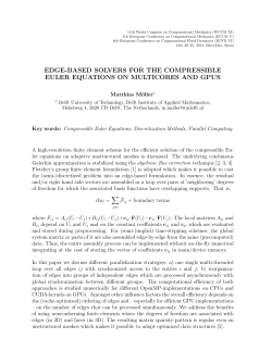
Before we give a detailed proof of the upper bound, let us sketch the
main ideas for the case s = 3. For simplicity, we will also assume p = 12 .
As we mentioned in the introduction, if we fix a set A1 of log4/3 n2 ≈
2 log4/3 n vertices with B1 = [n] − A1 , then G[A1 , B1 ] is a K3 -saturated
subgraph with about n log4/3 n edges. But we can do better than that (see
Figure 3.1):
So instead, we fix A1 to be a set of 2 log2 n vertices and add all edges
in G[A1 , B1 ] to our construction. This way we complete most of the edges
in B1 using about n log2 n edges. Of course, we still have plenty of edges
in G[B1 ] left incomplete, however, as we shall see, almost all of them are
induced by a small set B2 ⊆ B1 of size o(n). But then we can complete all
the edges in B2 using only o(n log n) extra edges: just take an additional set
A2 of log4/3 n2 vertices, and add all edges in G[A2 , B2 ] to our construction.
This way, however, we still need to take care of the Θ(n log n) incomplete
edges between A2 and B3 = B1 −B2 . As a side remark, let us point out that
dropping the K3 -freeness condition from K3 -saturation would make our life
easier here. Indeed, then we could have just chosen A2 to be a subset of
B2 .
The trick is to take yet another set A3 of o(log n) vertices, and add all
the o(n log n) edges of G between A3 and A2 ∪ B3 to our construction. Now
the o(log n) vertices in A3 are not enough to complete all the edges between
A2 and B3 , but if |A3 | = ω(1), then it will complete most of them. This
gives us a triangle-free construction on (1 + o(1))2 log2 n edges completing
all but o(n log n) edges, and by the observation above this is enough.
B1
B2
B3
A3
A1
A2
Figure 3.1: strong K3 -saturation
27
3.2. STRONG SATURATION
Let us now collect the ingredients of the proof. The next lemma says
that the graph comprised of the edges incident to a fixed set of a vertices
will complete all but an approximately (1 − p2 )a fraction of the edges in any
prescribed set E.
Lemma 3.2.4. Let s ≥ 3 be a fixed integer, and suppose a = a(n) grows to
infinity as n → ∞. Let A ⊆ [n] be a set of size a and E be a collection of
vertex pairs from B = [n] − A. Now consider the random graph GA defined
on [n] as follows:
1) GA [B] is empty,
2) GA [A] is a fixed graph such that any induced subgraph on
contains a copy of Ks−2 ,
a
log2 a
vertices
3) the edges between A and B are in GA independently with probability
p.
Then the expected
number of pairs in E that GA does not complete is at
a
most (1 − p2 )a− log a · |E|.
Proof. Suppose a pair {u, v} ∈ E of vertices is incomplete, i.e., adding the
edge uv to GA does not create a Ks . Because of the second condition, the
probability of this event can be bounded from above by the probability that
u and v have fewer than loga2 a neighbors in A. As the size of the common
neighborhood of u and v is distributed as Bin(a,
p2 ), Lemma 3.2.1 implies
a
that this probability is at most (1 − p2 )a− log a . This bound holds for any
pair in E, so
the expected number of bad pairs is indeed no greater than
a
(1 − p2 )a− log a · |E|.
A Ks -saturated graph cannot contain any cliques of size s. So if we
want to construct such a graph using Lemma 3.2.4, we need to make sure
that GA itself is Ks -free. The easiest way to do this is by requiring that
GA [A] do not contain any Ks−1 . In our application, GA will be a subgraph of
G(n, p), so in particular, we need GA [A] to be a subgraph of an Erdős-Rényi
random graph that is Ks−1 -free but induces no large Ks−2 -free subgraph.
Krivelevich [40] showed that whp we can find such a subgraph.
28
3.2. STRONG SATURATION
Theorem 3.2.5 (Krivelevich). Let s ≥ 3 be an integer, p ≥ cn−2/s (for
some small constant c depending on s) and G = G(n, p). Then whp G
contains a Ks−1 -free subgraph H that has no Ks−2 -free induced subgraph on
s−2
n s polylog n ≤ logn3 n vertices.
We will also use the fact that random graphs typically have relatively
small chromatic numbers (see e.g. [33]):
Claim 3.2.6. Let 0 < p < 1 be a constant and G = G(n, p). Then χ(G) =
(1 + o(1)) 2 log n n whp.
1/(1−p)
We are now ready to prove our main theorem.
Theorem 3.2.7. Let 0 < p < 1 be a constant, s ≥ 3 be a fixed integer
and G = G(n, p). Then whp G contains a Ks -saturated subgraph on (1 +
o(1))n log1/(1−p) n edges.
1
1
3
1
, β = 1−p
Proof. Define α = 1−p
2 , and set a1 = p (1 + log log n ) logα n,
α
a2
2
) logβ n2 and a3 = √log
a2 = (1 + log log
=
o(log
n).
Let
us
also
define
n
a2
β
A1 , A2 , A3 to be some disjoint subsets of [n] such that |Ai | = ai , and let
B1 = [n] − (A1 ∪ A2 ∪ A3 ).
Expose the edges of G[A1 ]. By Theorem 3.2.5 it contains a Ks−1 -free
subgraph G1 with no Ks−2 -free subset of size loga31a1 whp. Let H1 be the
graph on vertex set A1 ∪ B1 such that H1 [A1 ] = G1 , H1 [B1 ] is empty, and
H1 is identical to G between A1 and B1 . Now define B2 to be the set of
2
) logα n vertices
vertices in B1 that are adjacent to fewer than (1 + log log
αn
of A1 in the graph H1 . We claim that H1 completes all but O(n log log n)
of the vertex pairs in B1 not induced by B2 .
To see this, let F be the set of incomplete pairs in B1 not induced by
B2 . Now fix a vertex v ∈ B1 − B2 and denote its neighborhood in A1 by
2
Nv . By definition, |Nv | ≥ (1 + log log
) logα n. Let dF (v) be the degree of
αn
v in F , i.e., the number of pairs {u, v} ⊆ B2 that H1 does not complete.
Conditioned on Nv , the size of the common neighborhood of v and some
u ∈ B1 is distributed as Bin(|Nv |, p), so by Claim 3.2.1 the probability that
v|
is at most (1 − p)|Nv |−|Nv |/ log |Nv | ≤
this is smaller than loga31a1 ≤ log|N
2
|Nv |
(1 − p)logα n = n1 . On the other hand, if the common neighborhood contains
at least loga31a1 vertices in A1 , then it also induces a Ks−2 , thus the pair is
P
complete. Therefore E[dF (v)] ≤ 1 and E[ v∈B2 −B1 dF (v)] ≤ n.
29
3.2. STRONG SATURATION
P
Here the quantity v∈B2 −B1 dF (v) bounds |F |, the number of incomplete
edges in B1 that are not induced by B2 , so by Markov’s inequality this
number is indeed O(n log log n) whp. By the Observation above, we can
temporarily ignore these edges, and concentrate instead on completing those
induced by B2 . To complete them, we will use the (yet unexposed) edges
touching A2 .
The good thing about B2 is that it is quite small: For a fixed v ∈ B1 , the
size of its neighborhood in A1 is distributed as Bin(a1 , p), so the probability
2
αn
) logα n = pa1 − logloglog
is, by Claim 3.2.1,
that it is smaller than (1+ log log
n
n
2
α
α
at most e− logα n/4(log logα n) log1 n . So by Markov, |B2 |, the number of such
vertices, is smaller than logn n whp.
Now expose the edges of G[A2 ]. Once again, whp we can apply Theorem 3.2.5 to find a Ks−1 -free subgraph G2 that has no large Ks−2 -free
induced subgraph. Let H2 be the graph on A2 ∪ B2 such that H2 [A2 ] = G2 ,
H2 [B2 ] is empty, and H2 = G on the edges between A2 and B2 . Let us
apply Lemma 3.2.4 to GA2 = H2 with E containing all vertex pairs in B2 .
The lemma says that the expected number of incomplete pairs in E is at
most
a
|B2 |
n/
log
n
2 logβ (n
2 a2 − log2a2
)
2 ·
·
≤ (1 − p )
= o(1),
(1 − p )
2
2
so by Markov, H1 completes all of E whp, in particular it completes all the
edges in G[B2 ]. Note that |B2 | ≤ logn n also implies that H2 only contains
O(n) edges, so adding them to H1 does not affect the asymptotic amount
of edges in our construction.
However, the edges connecting A2 to B3 = B1 − B2 are still incomplete,
and there are Θ(n log n) of them, too many to ignore using the Observation.
The idea is to complete most of these using the edges between A3 and
A2 ∪ B3 , but we need to be a little bit careful not to create copies of Ks
with the edges in H2 [A2 ] = G2 . We achieve this by splitting up A2 into
independent sets.
a2
By Claim 3.2.6, we know that k = χ(G[A2 ]) = O log a2 , so G2 ⊆ G[A2 ]
can also be k-colored whp. Let A2 = ∪ki=1 A2,i be a partitioning into color
classes, so here G2 [A2,i ] is an empty graph for every i. Let us also split
A3 into 2k parts of size a4 = a3 /2k and expose the edges in G[A3 ]. Each
of the 2k parts contains a Ks−1 -free subgraph with no Ks−2 -free subset
30
3.3. WEAK SATURATION
of size loga34a4 with the same probability p0 , and by Theorem 3.2.5, p0 =
√
1 − o(1) (note that a4 = Ω( log a2 ) grows to infinity). This means that the
expected number of parts not having such a subgraph is 2k(1 − p0 ) = o(k),
so by Markov’s inequality, whp k of the parts, A3,1 , . . . A3,k , do contain such
subgraphs G3,1 , . . . , G3,k .
Now define H3,i to be the graph with vertex set A3,i ∪ A2,i ∪ B3 such that
H3,i [A3,i ] = G3,i , H3,i [A2,i ∪ B3 ] is empty, and the edges between A3,i and
A2,i ∪ B3 are the same as in G. Then we can apply Lemma 3.2.4 to show
that H3,i is expected to complete all but a (1 − p2 )a4 −a4 / log a4 fraction of the
A2,i -B3 pairs. This means that the expected number of edges between A2
and B3 that H3 = ∪ki=1 H3,i does not complete is bounded by
√
(1 − p2 )Ω(
log a2 )
√
· |A2 ||B3 | ≤ (1 − p2 )Ω(
log log n)
· O(n log n).
So if F 0 is the set of incomplete A2 -B3 edges, then another application of
Markov gives |F 0 | = o(n log n) whp.
It is easy to check that H = H1 ∪ H2 ∪ H3 is Ks -free, since it can be
obtained by repeatedly “gluing” together Ks -free graphs along independent
sets, and such a process can never create an s-clique. To estimate the size
of H, note that Claim 3.2.1 implies that whp all the vertices in A1 have
(1 + o(1))p|B1 | neighbors in B1 , so H1 contains (1 + o(1))n logα n edges.
We have noted above that H2contains O(n)
edges and H3 clearly contains
log
n
at most |A2 ∪ B3 ||A3 | = O n √log log n edges. So in total, H contains
(1 + o(1))n logα n edges.
Finally, the only edges H is not saturated at are either in F , in F 0 ,
touching A3 , or induced by A1 ∪ A2 . There are o(n log n) edges of each
of these four kinds, so any maximal Ks -free supergraph H 0 of H has (1 +
o(1))n logα n edges. This H 0 is Ks -saturated, hence the proof is complete.
3.3
Weak saturation
In this section we prove Theorem 3.1.3 about the weak saturation number
of random graphs of constant density. In fact, we prove the statement for a
slightly more general class of graphs, satisfying certain pseudorandomness
conditions. We will need some definitions to formulate this result.
31
3.3. WEAK SATURATION
Given a graph G and a vertex set X, a clique extension of X is a vertex
set Y disjoint from X such that G[Y ] is a clique and G[X, Y ] is a complete
bipartite graph. We define the size of this extension to be |Y |.
The following definition of goodness captures the important properties
needed in our proof.
Definition 3.3.1. A graph G is t-good with respect to γ if G satisfies the
following properties:
P1. For any vertex set X of size x and any integer y such that x, y ≤ t,
G contains at least γn disjoint clique extensions of X of size y.
P2. For any two disjoint sets S and T of size at least γn/2, there is a
vertex v ∈ T and X ⊆ S of size t − 1 such that X ∪ v induces a clique
in G.
It is not hard to see that the Erdős-Rényi random graphs satisfy the
properties:
Claim 3.3.2. Let 0 < p < 1 be a constant and let t be a fixed integer. Then
there is a constant γ = γ(p, t) > 0 such that whp G = G(n, p) is t-good with
respect to γ.
Proof. To prove property P1, fix x, y ≤ t and a set X of size x, and split
V −X
k groups of y elements (with some leftover): V1 , . . . , Vm where
j into
n−x
m = y . The probability that for some i ∈ [m], all the pairs induced
y+x
x
by V or connecting X and V are edges in G is p̃ = p( 2 )−(2) , which is a
i
i
constant. Let BX,y be the event that fewer than mp̃/2 of the Vi satisfy this.
By Claim 3.2.1, P(BX,y ) ≤ e−mp̃/8 .
2t
Now set γ = p( 2 ) /4t, then γn ≤ mp̃/2, so if BX,y does not hold then
there are at least γn different Vi ’s that we can choose
are
Yi wet log
the nsets
Pt tonbe
looking for. On the other hand, there are only x=0 x ≤ t t ≤ t · e n
choices for X and t choices for y, so
P(∪X,y BX,y ) ≤ t2 · et log n · e−γn/4 = o(1),
hence P1 is satisfied whp.
32
3.3. WEAK SATURATION
To prove property P2, notice that Theorem 3.2.5 implies that whp any
induced subgraph of G on at least logn3 n vertices contains a clique of size t.1
Let us assume this is the case and fix S and T . Then if a vertex v ∈ T has
at least logn3 n neighbors in S, then the neighborhood contains a t − 1-clique
in G that we can choose to be X. So if property P2 fails, then no such v
can have logn3 n neighbors in S.
The neighborhood of v in S is distributed as Bin(|S|, p), so the probability that v has fewer than logn3 n ≤ log|S|
neighbors in S is at most
2
|S|
(1 − p)|S|−|S|/ log |S| ≤ e−p|S|/2 ≤ e−pγn/4 by Claim 3.2.1. These events are
independent for the different vertices in S, so the probability that P2 fails
2
for this particular choice of S and T is e−Ω(n ) . But we can only fix S and
T in 22n different ways, so whp P2 holds for G.
Now we are ready to prove the following result, which immediately implies Theorem 3.1.3.
Theorem 3.3.3. Let G be 2s-good with respect to some constant γ. Then
s−1
w-sat(G, Ks ) = (s − 2)n −
.
2
Proof. To prove the lower bound on w-sat(G, Ks ), it is enough to show that
G is weakly saturated in Kn . Indeed, if H is weakly saturated in G and G
is weakly saturated in Kn , then H is weakly saturated in Kn : We can just
add edges one by one to H, obtaining G, and then keep adding edges until
we reach Kn in such a way that every added edge creates a new copy of Ks.
But then Theorem 3.1.2 implies that H contains at least (s − 2)n − s−1
2
edges, which is what we want.
Actually, G is not only weakly, but strongly saturated in Kn : property
P1 implies that for any vertex pair X = {u, v}, G contains a clique extension
of X of size s − 2. But then adding the edge uv to this subgraph creates
the copy of Ks that we were looking for.
Let us now look at the upper bound on w-sat(G, Ks ). Fix a core C of
s − 2 vertices that induces a complete graph (such a C exists by property
P1, as it is merely a clique extension of ∅ of size s−2). Our saturated graph
H will consist of G[C], plus s − 2 edges for each vertex v ∈ V − C, giving
1
We should point out that this statement is much weaker than Theorem 3.2.5 and
can be easily proved directly using a simple union bound argument.
33
3.3. WEAK SATURATION
s−1
a total of s−2
+
(s
−
2)(n
−
s
+
2)
=
(s
−
2)n
−
edges. We build H
2
2
in steps.
Let V 0 be the set of vertices v ∈ V − C adjacent to all of C. Note
that |V 0 | ≥ γn by property P1. We start our construction with the graph
H0 ⊆ G on vertex set V0 = C ∪ V 0 that contains all the edges touching C.
Once we have defined Hi−1 on Vi−1 , we pick an arbitrary vertex vi ∈
V − Vi−1 , and choose a set Ci ⊆ Vi−1 of s − 2 vertices that induces a clique
in G with vi . Again, we can find such a Ci as a clique extension of vi ∪C. In
fact, by the definition of V 0 , this Ci will lie in V 0 . Then we set Vi = Vi−1 ∪ vi
and define Hi to be the graph on Vi that is the union of Hi−1 and the s − 2
edges connecting vi to Ci . Repeating this,
end up with some
we eventually
graph H = Hl on V = Vl that has n2 − n−s+2
edges.
We claim it is
2
saturated.
C
vi
Vi−1
Ci
Figure 3.2: Weak K4 -saturation. Black edges are in H, gray edges are in G
but not in H.
We really prove a bit more: we show, by induction, that Hi is weakly
Ks -saturated in G[Vi ] for every i. This is clearly true for i = 0: any edge of
G[V0 ] not contained in H0 is induced by V 0 , and forms an s-clique with C.
Now assume the statement holds for i − 1. We want to show that we
can add all the remaining edges in Gi = G[Vi ] to Hi one by one, each time
creating a Ks . By induction, we can add all the edges in Gi−1 , so we may
assume they are already there. Then the only missing edges are the ones
touching vi .
If v ∈ Vi is a clique extension of Ci ∪ vi then adding vvi creates a Ks , so
we can add this edge to the graph. Property P1 applied to C ∪Ci ∪vi to find
34
3.4. FURTHER REMARKS
clique extensions of size 1 shows that there are at least γn such vertices.
Let N be the new neighborhood of vi after these additions, then |N | ≥ γn.
Now an edge vvi can also be added if v ∪C 0 induces a complete subgraph
in G, where C 0 is any s − 2-clique in Gi [N ]. Let us repeatedly add the
available edges (updating N with every addition). We claim that all the
missing edges will be added eventually.
Suppose not, i.e., some of the edges in Gi touching vi cannot be added
using this procedure. There cannot be more than γn/2 of them, as that
would contradict property P2 with S = N and T being the remaining
neighbors of vi in Vi . But then take one such edge, vvi , and apply property
P1 to C ∪ {v, vi }. It shows that there are γn disjoint clique extensions of
size s−2, that is, γn disjoint s−2-sets in V 0 that form s-cliques with {v, vi }.
But at most γn/2 of these cliques touch a missing edge other than
vvi , so there is a C 0 among them that would have been a good choice for
v. This contradiction establishes our claim and finishes the proof of the
theorem.
3.4
Further remarks
Many of the saturation results also generalize to hypergraphs. For example,
n
r
r
r
r
Bollobás
[9]
and
Alon
[1]
proved
that
sat(K
,
K
)
=
w-sat(K
,
K
)
=
−
n
s
n
s
r
n−s+r
r
,
where
K
denotes
the
complete
r-uniform
hypergraph
on
t
vertices.
t
r
It would therefore be very interesting to see how saturation behaves in
Gr (n, p), the random r-uniform hypergraph.
With some extra ideas, our proofs can be adapted to give tight results
r
-saturated hypergraphs, but the general Ksr -saturated case apabout Kr+1
pears to be more difficult. It is possible, however, that our methods can
be pushed further to solve these questions, and we plan to return to the
problem at a later occasion.
Another interesting direction is to study the saturation problem for nonconstant probability ranges. For example, Theorem 3.1.1 about strong sat1
1
≤ p ≤ 1 − o(n)
in a fairly
uration can be extended to the range logε(s)
n
straightforward manner. As for K3 -saturation, a bit of extra work yields the
correct asymptotics in the range n−1/2+ε ≤ p 1, as well. Here we can show
that sat(G(n, p), K3 ) = (1 + o(1)) np log np2 . Note also that for p n−1/2
there are much fewer triangles in G(n, p) than edges, so any saturated graph
35
3.4. FURTHER REMARKS
must contain almost all the edges, i.e., sat(G(n, p), K3 ) = (1 + o(1)) n2 p.
These results give us a fairly good understanding of K3 -saturation in random graphs. However, in general, Ks -saturation for sparse random graphs
appears to be more difficult, and it seems that for p much smaller than log1 n
the saturation numbers will depend on s.
It is also not difficult to extend our weak saturation result, Theorem 3.1.3, to the range n−ε(s) ≤ p ≤ 1. A next step could be to obtain results
for smaller values of p, in particular, it would be nice to determine the ex
act probability range where the weak saturation number is (s − 2)n − s−1
.
2
Note that our lower bound holds as long as G(n, p) is weakly Ks -saturated
in Kn . This problem was studied by Balogh, Bollobás and Morris [4], who
showed that the probability threshold for G(n, p) to be weakly Ks -saturated
(2s)−2
. It might be possible
is around p ≈ n−1/λ(s) polylog n, where λ(s) = s−2
that w-sat(G(n, p), Ks ) changes its behavior at the same threshold.
F -saturation in the complete graph has been studied for various different graphs F (see [27] for references). For example, Kászonyi and Tuza
[37] showed that for any fixed (connected) graph F on at least 3 vertices,
sat(n, F ) is linear in n. As we have seen, this is not true in G(n, p). However, analogous results in random host graphs could be of some interest.
36
Chapter 4
A random triadic process
4.1
Introduction
The principle of triadic closure is an important concept in social network
theory (see e.g. [20]). Roughly speaking, it says that when new friendships
are formed in a social network, it is more likely to occur between two people
sharing a common friend, thus “closing” a triangle, than elsewhere. We
will consider a simplistic model of the evolution of a social network, where
friendships can only be formed through a common friend, and triadic closure
eventually occurs at any triangle with probability p, independently of other
triangles. We refer to this process as the triadic process.
Formally, let H = H(n, p) be a random 3-uniform hypergraph on [n]
where each triple independently appears with probability p. The triadic
process is the following graph process. We start with the star G0 on the
same vertex set [n], containing all the edges incident to some vertex v0 , and
repeatedly add any edge xy if there is a vertex z such that xz and zy are
already in the graph and xzy ∈ H. We say that the process propagates if
all the edges are added to the graph eventually. It is easy to see that this
event does not depend on the order the edges are added in. In this chapter
we prove that the threshold probability for propagation is 2√1 n .
Theorem 4.1.1. Suppose p =
√c ,
n
for some constant c > 0. Then,
1) If c > 12 , then the triadic process propagates whp.
√
2) If c < 12 , then the triadic process stops at O(n n) edges whp.
37
4.1. INTRODUCTION
As usual, we say that some property holds with high probability or whp
if it holds with probability tending to 1 as n tends to infinity.
Randomized graph processes have been intensively studied in the past
decades. One notable example is the triangle-free process, originally motivated by the study of the Ramsey number R(3, n) (see e.g. [26]). In this
process the edges are added one by one at random as long as they do not
create a triangle in the graph. The triadic process is a slight variant of
this, with a very similar nature. Indeed, our analysis makes good use of the
tools developed by Bohman [7] when he applied the differential equation
method to track the triangle-free process. Several other related processes
were also analyzed using differential equations, e.g. [8]. For more information about this method we refer the interested reader to the excellent
survey of Wormald [54].
Coja-Oghlan, Onsjö and Watanabe [17] investigated a similar kind of
closure while analyzing connectivity properties of random hypergraphs.
They say that a 3-hypergraph is propagation connected if its vertices can
be ordered in some way v1 , . . . , vn so that each vi (i ≥ 3) forms a hyperedge
with two preceding vertices. They obtain the threshold probability for the
propagation connectivity of H(n, p) up to a small multiplicative constant.
Using this directed notion of connectivity, our problem asks when the random 3-hypergraph on the line graph of Kn is propagation connected from
the star.
Our main motivation for considering the triadic process comes from
the theory of random 2-dimensional simplicial complexes.
A simplicial 2
V
complex on the vertex set V is a set family Y ⊆ ≤3
closed under taking
subsets. The dimension of a simplex σ ∈ Y is defined to be |σ| − 1. We
use the terms vertices, edges and faces for 0, 1 and 2-dimensional simplices,
respectively. The 1-skeleton of a 2-complex is the subcomplex containing
its vertices and edges.
The Linial–Meshulam model of random simplicial complexes, introduced
in [41], is a generalization of the Erdős–Rényi random graph model and has
been studied extensively in recent years. The random 2-complex Y2 (n, p) is
defined to have the complete 1-skeleton, i.e., all vertices and edges, and each
of the faces independently with probability p. The study of random complexes involves both topological invariants and combinatorial properties,
including homology groups, homotopy groups, collapsibility, embeddability
and spectral properties.
38
4.1. INTRODUCTION
One of the oldest questions of this kind, asked by Linial and Meshulam
[41], is how the fundamental group π1 (Y2 (n, p)) of the random 2-complex
behaves. Babson, Hoffman and Kahle [3] showed that if p < n−α for some
arbitrary α > 1/2 then the fundamental group is nontrivial whp.
p On the
other hand, they proved that π1 (Y2 (n, p)) is trivial for p > 4 log n/n,
which means that the threshold probability for being simply connected
should be close to n−1/2 . As a corollary of the first part of Theorem 4.1.1,
we improve the upper bound on the threshold probability.
Corollary 4.1.2. Let p =
simply connected whp.
√c
n
for some constant c > 12 . Then Y2 (n, p) is
Proof. Suppose we have a 2-complex C such that one of its edges, e, is
contained in a unique face f . Then we can collapse f onto the other two
edges without changing the fundamental group of C. In fact, C − f −
e is homotopy equivalent to C, the former complex being a deformation
retract of the latter. We say that a 2-complex with complete 1-skeleton is a
collapsible hypertree if we can apply a sequence of collapses to it and end up
with a tree. Clearly, a collapsible hypertree has trivial fundamental group.
Now observe that Theorem 4.1.1 implies that Y2 (n, p) contains a collapsible hypertree whp. Indeed, if the process propagates, then take C to
be the subcomplex of the faces that correspond to the triples we used to add
edges to the graph. Then by definition, the reverse of the triadic process
on C is exactly a sequence of collapses resulting in a star.
Basic results about the topology of complexes tell us that the addition
of faces to a simply connected complex does not change the fundamental
group, hence π1 (Y2 (n, p)) is trivial whp.
After the publication of this result, we learned that Gundert and Wagner
[32] independently improved the bound in [3], and showed that Y2 (n, p) is
whp simply connected for p = √cn where c is a sufficiently large constant.
4.1.1
Proof outline
Instead of exposing all the triples at once, we will be sampling them on
the fly, trying to extend the edge set of the graph. Both the proofs of
the upper bound and the lower bound consist of two phases. In the first
phase we make one step at a time: we choose, uniformly at random, one
(yet unsampled) triple spanning exactly two edges and expose it. With
39
4.2. THE DIFFERENTIAL EQUATION METHOD
probability p the triple is selected, hence we can add the third edge to
our edge set. The second phase proceeds in rounds: we simultaneously
expose all the unsampled triples spanning two edges, and extend the edge
set according to the outcome.
The essence of the proof is to track the behavior of certain variables
throughout the process. As we will see, this is not a very hard task to
do in the second phase, using standard measure concentration inequalities.
However, during the initial phase of the process, the codegrees (one of the
variables we track) are not concentrated, which forces us to do a more
careful analysis of the beginning of the process. For this we will use the
differential equation method.
We organize the rest of the chapter as follows. In Section 4.2 we give
an overview of how we apply the differential equation method. A detailed
analysis of the actual implementation follows in Section 4.3. We move on
to the second phase of the process in Section 4.4, thereby completing the
proof of Theorem 4.1.1. We finish with some remarks in Section 4.5.
Notations: Throughout the chapter, we will omit floor and ceiling signs
whenever they are not necessary. The sign ± will be used to represent both
a two-element set of values and a whole interval, but it should be clear from
the context which one is the case.
4.2
The differential equation method
At any point in the process, we say that a vertex triple {u, v, w} is open if it
spans exactly two edges but has not yet been sampled. We will also use the
notation uvw for an open triple with edges uv and vw. By an open triple
at u, we mean a triple uvw, i.e., one that has its missing edge adjacent to
the vertex u.
In each step, our process picks an open triple uniformly at random and
samples it. If the answer is positive then we close the triple by adding the
missing edge to the graph. To analyze this process we apply the differential
equation method, using some ideas from [7].
For simplicity, let us denote the graph we obtain after i samples by
Gi . We consider the following random variables: Dv (i) is the degree of the
vertex v in Gi . Fv (i) is the number of open triples at v, so it is the number
40
4.2. THE DIFFERENTIAL EQUATION METHOD
of ways for v to gain a new incident edge in Gi+1 . Xu,v (i) is the codegree
of u and v, i.e., the number of common neighbors of u and v in Gi .
To provide some insight, we first heuristically describe the process. Let
us assume for now that the Dv (i) are concentrated around some value D(i),
and similarly the Fv (i) are approximately equal to some value F (i). We
further assume that the variables are very close to their expectations.
In step i + 1 we choose an open triple uniformly at random, so each
triple is chosen with probability P F2 v (i) ≈ nF2(i) , and then sample it. With
v
probability p the sample is successful, hence we can close the triple. As the
number of open triples at a vertex v is about F (i), the change in the degree
of a vertex v we expect to see is
D(i + 1) − D(i) ≈
2p
.
n
Now let us see how Fv (i) is affected by a step. We gain open triples
at v either if we successfully sample one of them (adding the edge vw),
in which case new open triples are formed with the neighbors of w, or
if we successfully sample a triple at some neighbor of v. On the other
hand, we lose the sampled triple regardless of the outcome. The probability
≈ n2 , so
of sampling an open triple at some specific vertex w is P2FwF(i)
v v (i)
assuming all the codegrees are negligible compared to D(i), the expected
change is
2
F (i + 1) − F (i) ≈ (2pD(i) − 1).
n
To smooth out this discrete process, we introduce a continuous variable
t and say that step i corresponds to time t = ti = ni2 . Let us also rescale
D and F by considering the smooth
√ functions d and f in t, where we want
d(t) to be approximately√D(i)/ n and f (t) to be approximately F (i)/n.
Note that, since p = c/ n, our assumptions so far suggest the following
behavior:
d(t + 1/n2 ) − d(t)
d (t) ≈
≈ n3/2 (D(i + 1) − D(i)) ≈ 2c
2
1/n
0
and
f 0 (t) ≈
f (t + 1/n2 ) − f (t)
≈ n(F (i + 1) − F (i)) ≈ 4cd(t) − 2.
1/n2
41
4.2. THE DIFFERENTIAL EQUATION METHOD
Let us emphasize that this little musing that we are presenting here
is not a proof at all — a detailed analysis and the proof of concentration
will follow in Section 4.3. However, it at least indicates why it is plausible
to believe that the actual values of Dv (i) and Fv (i) follow the trajectories
of d and f given by the system of differential equations d0 (t) = 2c and
f 0 (t) = 4cd(t) − 2.
In the previous paragraphs we made the assumption that the codegrees
are negligible compared to the degrees, but since they are not concentrated,
proving this still needs some thought. To this end, we introduce two more
random variables. Yu,v (i) denotes the number of open 3-walks uww0 v from u
to v, i.e., 3-walks where we require that uww0 be open (but allowing w = v),
and Zu,v (i) is the number of open 4-walks uww0 w00 v (again, allowing vertex
repetitions), where both uww0 and w0 w00 v are open. Note that Yu,v is not
symmetric in u and v.
The point is that Yu,v and Zu,v are concentrated (as we will see in Section
4.3), and — amazingly enough — their one-step behavior can be described
with fairly simple formulas. So let us continue with our thought experiment
and assume that all Yu,v (i) ≈ Y (i), all Zu,v (i) ≈ Z(i), and all variables are
close to their expectations.
First of all, the increase in the codegrees comes from a successful sample
in a 3-walk, so we expect
Xu,v (i + 1) − Xu,v (i) ≈
4cy(t)
2p(Yu,v (i) + Yv,u (i))
≈ 2
.
nF (i)
n f (t)
This will be enough to prove a uniform O(log n) upper bound over all the
codegrees, so we can keep ignoring the effect of X in the next few paragraphs.
Let us look at the change in Yu,v (i). There are three different ways a
new open 3-walk uww0 v can appear after step i+1, depending on which one
of uw, ww0 and w0 v is the new edge. When uw is the new edge, there is a
4-walk utww0 v in Gi where utw is open. We can count such configurations
by first choosing w0 as a neighbor of v and then choosing an open 3-walk
utww0 . Note that for any such choice, uww0 will be an open triple in Gi+1 ,
except if w0 is the same as u, or a common neighbor of u and w. The latter
cases are negligible, so there are about Y (i)D(i) possibilities in this case.
Similarly, when ww0 is the new edge, new 3-walks come from 4-walks
uwtw0 v, and we can count the number of options by first choosing w as a
42
4.2. THE DIFFERENTIAL EQUATION METHOD
neighbor of u and then an open 3-walk from w to v. Again, the triple uww0
will be open in Gi+1 if w0 is neither u, nor a common neighbor of u and v,
so we find Y (i)D(i) possibilities of this type. Finally, w0 v can only be the
new edge if w0 tv was successfully sampled in some open 4-walk uww0 tv, so
there are about Z(i) such options.
On the other hand, we lose an open 3-walk if we sample its open triple,
whether or not the sample is successful. As any particular triple is chosen
with probability about nF2(i) , this means that we expect to see
2 Y (i + 1) − Y (i) ≈
p 2Y (i)D(i) + Z(i) − Y (i) .
nF (i)
The change in Z(i) is a bit easier to analyze: Once again, we obtain a
new 4-walk uww0 w00 v if one of its edges is added in step i+1. We will assume
it is the first edge, uw, but by symmetry our counting argument works for
all other edges, as well. Then the 4-walk comes from a 5-walk utww0 w00 v
in Gi . We can count the number of options by first taking an open triple
vw00 w0 at v and then choosing an open 3-walk from u to w0 . Again, the
created 4-walk will automatically be open unless w0 is u or a neighbor of u,
so there are about Y (i)F (i) candidates of this type and 4Y (i)F (i) in total.
And then of course, we lose an open 4-walk if we sample one of its two open
triples, regardless of the outcome. This suggests
2 4pY (i)F (i) − 2Z(i) .
Z(i + 1) − Z(i) ≈
nF (i)
Once again, we are looking
√ for smooth functions y and z such that
y(t) is approximately Y (i)/ n and z(t) is about Z(i)/n. Then the same
computation as before gives the differential equations
y 0 (t) =
2
(2cd(t) − 1)y(t) + cz(t)
f (t)
and
z 0 (t) =
4
2cy(t)f (t) − z(t) .
f (t)
We have yet to talk about the initial conditions of the above system
of differential equations. Our process starts with a star centered at some
vertex v0 , i.e., an n-vertex graph with n − 1 edges, all of them touching v0 .
43
4.3. CALCULATIONS
Then Dv (0) = 1, Fv (0) = n − 2, Yu,v (0) = 0 and Zu,v (0) = n − 3 for any two
vertices u and v other than v0 . For convenience, we will drop the center of
the star from consideration in the sense that we do not define the variables
with v0 among the indices. This is a technicality that allows us to prove
concentration, and since our recurrence relations never use those variables,
it causes no problem.
Hence we obtain the initial conditions d(0) = 0, f (0) = 1, y(0) = 0 and
z(0) = 1, and an easy calculation shows that the corresponding solution of
our system of differential equations is
f (t) = 1 − 2t + 4c2 t2
z(t) = f 2 (t).
d(t) = 2ct
y(t) = d(t)f (t)
In the next section we prove that the variables indeed closely follow the
paths defined by these functions.
4.3
Calculations
In this section we show that our variables follow the prescribed trajectories
up to some time T . Of course, we cannot hope to do so if f (t) vanishes
somewhere on [0, T ], as that would mean that the process is expected to
die before time T . Now if c > 1/2
√ then f has no positive root, so this is
not an issue: we can take T √
= log n. However, if c ≤ 1/2 then f does
1− 1−4c2
reach 0, first at time T0 =
. In this case T will be chosen to be a
4c2
constant arbitrarily close to T0 .
The allowed deviation of each variable will be defined by one of the error
functions
g1 (t) = eKt n−1/6
where
g2 (t) = (1 + d(t))eKt n−1/6 ,
and
1
d(t)
+
.
K = 100 · max 1 +
0≤t≤T
f (t) f (t)
It is clearly enough to prove the first part of Theorem 4.1.1 for c ≤ 1,
so from now on we will assume this is the case.
Let us define Gi to be the event that all of the bounds below in Proposition 4.3.1(a)-(e) hold for every pair of vertices u and v and for all indices
j = 0, . . . , i. This section is devoted to the proof of the following result,
which is the key to proving that the variables follow the desired trajectories.
44
4.3. CALCULATIONS
Proposition 4.3.1. Fix some vertices u and v. Then, conditioned on Gj−1 ,
each of the following bounds fails with probability at most n−10 .
√
(a) Dv (j) ∈ d(tj ) ± g1 (tj ) n
(b) Fv (j) ∈ f (tj ) ± g1 (tj ) n
(c) Xu,v (j) ≤ 50 log n
√
(d) Yu,v (j) ∈ y(tj ) ± g2 (tj ) n
(e) Zu,v (j) ∈ z(tj ) ± g2 (tj ) n
As a corollary, we obtain our main result.
√
Theorem 4.3.2. Suppose c ≤ 1, and T ≤ log n and K are defined as
above. Then the bounds in Proposition 4.3.1(a)-(e) hold with high probability for all vertices u and v and for every j = 0, . . . , T · n2 .
Proof. It is easy to check that G0 always holds. If Bj is the event that,
conditioned on Gj−1 , at least one of these bounds fails for j, then the failure
T n2
probability is exactly P[∪j=1
Bj ]. A trivial union bound over all pairs of
vertices and all equations in Proposition 4.3.1 shows that P[Bj ] ≤ 5n−8 ,
n2
hence another union bound over the indices gives P[∪Tj=1
Bj ] ≤ n−5 = o(1).
To prove Proposition 4.3.1, we follow the strategy in [7] and analyze each
random variable separately. Our plan is to use some martingale concentration inequalities to bound the probability of large deviation. However, since
we cannot track the exact values of the expectations, only estimate them by
some intervals, we will use two separate sequences to bound each variable:
A submartingale to bound from below, and a supermartingale to bound
from above.
Recall that a stochastic process X0 , X1 , . . . is called a submartingale if E[Xi+1 |X1 , . . . , Xi ] ≥ Xi for all i, and a supermartingale if
E[Xi+1 |X1 , . . . , Xi ] ≤ Xi for all i. We say that a sequence X0 , X1 , . . . of
variables is (η, N )-bounded if Xi − η ≤ Xi+1 ≤ Xi + N for all i. We
call a sequence of pairs X0± , X1± , . . . an (η, N )-bounded martingale pair,
if X0+ , X1+ , . . . is an (η, N )-bounded submartingale and X0− , X1− , . . . is an
(η, N )-bounded supermartingale. The following concentration results of
Bohman [7] are essential for proving that the variables follow the desired
trajectories:
45
4.3. CALCULATIONS
Lemma 4.3.3 (Bohman). Suppose η ≤ N/10 and a < ηm.
X0± , X1± , . . . is an (η, N )-bounded martingale pair then
a2
+
P[Xm
≤ −a] ≤ e− 3ηmN
and
If 0 ≡
a2
−
P[Xm
≥ a] ≤ e− 3ηmN .
The general idea for analyzing a random variable R(i), representing any
of the above five variables, is the following. In step i, an open triple is
sampled, and thus with probability p a new edge is added to our graph. We
split the one-step change in R(i) into two non-negative
P variables: Ai is the
gain and Ci is the loss in step i, so R(j) = R(0) + ji=1 Ai − Ci . The gain
comes from the contribution of the added edge after a successful sample.
Loss can only occur when some open triple stops being open, either because
it was sampled or because its missing edge was added through some other
open triple (although the effect of the latter event is negligible compared to
the former if the codegrees are small).
Next we estimate the expectation of Ai (using the recurrence relations
−
we hinted at in Section 4.2), so that we can define A+
i and Ai , shifted
copies of Ai with P
non-negative and non-positive expectations, respectively.
±
This way Bj = ji=1 A±
i is an (η, N )-bounded martingale pair, where η
is approximately the expectation and N is some trivial upper bound on
Ai . We
do the same with the Ci to define Ci± and the martingale pair
P
j
Dj± = i=1 Ci± .
Finally
=
Pj we establish a connection between the concentration of R(j)
±
R(0) + i=1 Ai − Ci and the concentration of our shifted variables Bj and
Dj± in Lemma 4.3.7, and then use the concentration of martingale pairs,
Lemma 4.3.3, to bound the error probabilities in Corollary 4.3.8.
The rest of this section is devoted to the actual calculations. The reader
might want to skip the details at a first reading. The first subsection establishes the tools we use to prove concentration, while the remaining five
subsections prove one by one the five parts of Proposition 4.3.1.
4.3.1
Tools
The following claim will help us clean up the calculations
of the expecta
d(t)
1
tions. Recall that K = 100 · max0≤t≤T 1 + f (t) + f (t) .
46
4.3. CALCULATIONS
Claim 4.3.4. Let 0 ≤ t ≤ T so that f (t) > 0 is bounded away from 0 (t
might depend on n). If r(t) is one of the functions 1, d(t) or f (t) then the
following inequalities hold:
√ n)
(r(t) ± g1 (t))(f (t) ± g1 (t)) 1 + O( log
n
K
⊆ r(t) ± g1 (t),
f (t) ± g1 (t)
20
2
√ n)
(r(t) ± g1 (t))(y(t) ± g2 (t)) 1 + O( log
n
K
⊆ r(t)d(t) ± g2 (t),
f (t) ± g1 (t)
20
log
n
(z(t) ± g2 (t)) 1 + O( √n )
K
⊆ f (t) ± g2 (t).
f (t) ± g1 (t)
20
Proof. Straightforward calculus shows that
2 1
1
g1 (t)
g1 (t)
⊆
± 2 +O
.
f (t) ± g1 (t)
f (t) f (t)
f 3 (t)
Using this, we will multiply out the formulas on the left-hand side of the
inequalities. Note that g1 (t) and g2 (t) are both O(n−1/7 ), so in the expanded
formulas, any term containing two factors of the type gα (t) or a factor of
√ n ) is consumed by an O(n−2/7 ) error term. Hence the left-hand
O( polylog
n
side of the first inequality is contained in
log n
1
g1 (t)
−2/7
(r(t) ± g1 (t))(f (t) ± g1 (t)) 1 + O( √ )
±
+ O(n
)
f (t) f 2 (t)
n
2r(t)
K
⊆ r(t) ±
+ 1 g1 (t) + O(n−2/7 ) ⊆ r(t) ± g1 (t).
f (t)
20
Similarly, the left-hand side of the second inequality is contained in
log2 n
1
g1 (t)
−2/7
(r(t) ± g1 (t))(y(t) ± g2 (t)) 1 + O( √ )
±
+ O(n
)
f (t) f 2 (t)
n
r(t)
y(t)
r(t)y(t)
⊆ r(t)d(t) ±
+
+
g2 (t) + O(n−2/7 )
f (t) f (t)(1 + d(t)) f 2 (t)(1 + d(t))
K
⊆ r(t)d(t) ± g2 (t)
20
47
4.3. CALCULATIONS
using y(t) = f (t)d(t) and g2 (t) = (1 + d(t))g1 (t). Finally, the left-hand side
of the last inequality is contained in
g1 (t)
log n
1
−2/7
±
+ O(n
)
(z(t) ± g2 (t)) 1 + O( √ )
f (t) f 2 (t)
n
1
z(t)
⊆ f (t) ±
+
g2 (t) + O(n−2/7 )
f (t) f 2 (t)(1 + d(t))
K
⊆ f (t) ± g1 (t)
20
using z(t) = f 2 (t).
The remaining lemmas connect the concentration of the original variables and those shifted by the expectations. We will use the following
observations in the calculations.
Claim 4.3.5. Let s(t) be a differentiable function on [0, T ] such that
supt∈[0,T ] |s0 (t)| = O(polylog n) and ti = ni2 . Then
Z tj
j−1
1 X
s(τ )dτ + O(n−1 ).
s(ti ) =
n2 i=0
0
Proof. It is a well-known fact in numerical analysis that for reals a ≤ q ≤ b
Z b
≤ (b − a)2 sup |s0 (t)|.
s(τ
)dτ
−
(b
−
a)s(q)
t∈[a,b]
a
Taking a = q = ti with b = ti+1 and using ti+1 − ti = n12 , this gives
Z ti+1
ti+1 − ti
s(t
)
i
s(τ )dτ − 2 ≤
sup |s0 (t)|,
n
n2
t∈[ti ,ti+1 ]
ti
and summing these up for i = 0, . . . , j − 1, we get
Z
j−1
0
tj
tj · sup
X
1
t∈[0,tj ] |s (t)|
s(t
)
≤
s(τ
)dτ
−
i 0
n2 i=0
n2
polylog n
=O
≤ O(n−1 ).
2
n
48
4.3. CALCULATIONS
This claim will be applied when s is one of the functions d0 , f 0 , x0 , y 0 , z 0 , g10
and√g20 , in which case s0 is indeed bounded by O(polylog n) in the interval
[0, log n].
Claim 4.3.6. For α ∈ {1, 2} we have
Z t
1
gα (τ )dτ ≤ (gα (t) − n−1/6 ).
K
0
Proof. Note that gα (t) = ϕ(t)eKt n−1/6 , where ϕ(t) is either constant 1 or
1 + d(t). In both cases, ϕ(0) = 1 and ϕ0 (t) ≥ 0 for t ≥ 0, so
0
1
gα0 (t)
Kt −1/6
=
ϕ(t)e n
= (ϕ0 (t)eKt /K + ϕ(t)eKt )n−1/6 ≥ gα (t).
K
K
Hence
Z
t
Z
gα (τ )dτ ≤
0
0
t
gα0 (τ )
1
dτ = (gα (t) − n−1/6 ),
K
K
as required.
It is time to formally define the shifted variables. Recall that if R(i)
represents one of our random variables, then we use the non-negative variables Ai and Ci for the one-step increase and decrease in R, respectively,
so that R(i) − R(i − 1) = Ai − Ci . Our aim is to show that R(i) is approximately nγ r(ti ) for some real γ, where the error (the allowed fluctuation of
R) is bounded by nγ gα (ti ) for some α ∈ {1, 2}. Here our choice of γ and α
depends on the variable R represents: γ will be 1 for F and Z, 1/2 for D
and Y , and 0 for X, while α will be 1 for D and F , and 2 for X, Y and Z.
To show the concentration of R, we approximate Ai and Ci by their
expectations, which, as we shall prove, lie in the intervals nγ−2 (rA (ti−1 ) ±
K
g (t )) and nγ−2 (rC (ti−1 ) ± K2 gα (ti−1 )), respectively, for some appro2 α i−1
priately chosen functions rA (t) and rC (t). Thus we can define the shifted
+
−
variables A+
i and Ci having non-negative expectation, as well as Ai and
Ci− having non-positive expectation as follows:
A±
i
γ−2
= Ai − n
K
(rA (ti−1 ) ∓ gα (ti−1 ))
2
with
K
gα (ti−1 ))
2
with
Ci± = Ci − nγ−2 (rC (ti−1 ) ∓
49
Bj±
=
j
X
A±
i
i=1
j
Dj± =
X
i=1
Ci± .
and
4.3. CALCULATIONS
P
Lemma 4.3.7. Suppose the variable R satisfies R(j) = nγ r(0) + ji=1 Ai −
Ci , where r is a polynomial in t such that r0 (t) = rA (t) − rC (t). Then
R(j) ≤ nγ (r(tj ) + gα (tj )) − nγ−1/6 /2 + Bj− − Dj+
γ
R(j) ≥ n (r(tj ) − gα (tj )) + n
γ−1/6
/2 +
Bj+
−
and
Dj− .
Proof. Let us first consider the upper bound:
γ
R(j) = n r(0) +
j
X
A i − Ci
i=1
j
X
K
−
γ−2
= n r(0) +
Ai + n (rA (ti−1 ) + gα (ti−1 ))
2
i=1
j X
K
+
γ−2
−
Ci + n (rC (ti−1 ) − gα (ti−1 ))
2
i=1
γ
= Bj− − Dj+ + nγ r(0)
+n
γ−2
j
X
(rA (ti−1 ) − rC (ti−1 )) + n
γ−2
i=1
j
X
Kgα (ti−1 )
i=1
Now we apply Claim 4.3.5 with functions rA (t) − rC (t) (a polynomial) and
Kg
√ α (t) (a product of a polynomial and an exponential function). As T ≤
log n, their derivatives are clearly bounded by O(polylog n) on [0, T ].
R(j) ≤ Bj− − Dj+ + nγ r(0)
Z tj
Z
γ
γ
+n
(rA (τ ) − rC (τ ))dτ + n
0
γ
≤ n (r(tj ) + gα (tj )) − n
tj
Kgα (τ )dτ + O(n−1 )
0
γ−1/6
/2 +
Bj−
− Dj+
using Claim 4.3.6 and nγ−1/6 + O(n−1 ) ≥ nγ−1/6 /2 in the last step.
The lower bound comes from an analogous argument by changing the
appropriate signs.
Using this, we can estimate the probability that R(j) deviates from its
expectation:
50
4.3. CALCULATIONS
Corollary 4.3.8. Suppose the numbers γ, α and the functions R, r, rA , rC
satisfy the conditions of Lemma 4.3.7. Suppose furthermore that Bj± and
Dj± are (η1 , N1 )-bounded and (η2 , N2 )-bounded martingale pairs, respectively, where ηβ Nβ ≤ ε and ηβ < Nβ /10 for β = 1, 2. Then the probability
that R(j) 6∈ nγ (r(tj ) ± gα (tj )) is at most 4e−
n2γ−1/3
50εj
.
Proof. Lemma 4.3.7 shows that R(j) > nγ (r(tj )+gα (tj )) implies nγ−1/6 /2 <
Bj− −Dj+ , hence this event is contained in the union of the events nγ−1/6 /4 <
Bj− and −nγ−1/6 /4 > Dj+ . A straightforward application of Lemma 4.3.3
then gives a bound of e−
n2γ−1/3
50εj
on the probability of each event, thus R(j) >
n2γ−1/3
nγ (r(tj ) + gα (tj )) occurs with probability at most 2e− 50εj . A similar
argument using the other inequality of Lemma 4.3.7 gives the same bound
on the probability of the event R(j) < nγ (r(tj ) − gα (tj )), finishing the
proof.
4.3.2
Degrees
Recall that in this section, and also in the next four sections, we assume Gj−1
holds, i.e., the values of Dv , Fv , Xu,v , Yu,v and Zu,v are all in the prescribed
intervals during the first j − 1 steps.
Proof of Proposition 4.3.1(a). Let Ai be the indicator random variable of
the eventP
that an open triple at v was successfully sampled in step i. Then
Dv (j) = ji=1 Ai . The probability that Ai+1 = 1 is
2c(f (ti ) ± g1 (ti ))
1
2pFv (i)
K Kti −1/6
P
∈ 3/2
⊆ 3/2 2c ± e n
n (f (ti ) ± g1 (ti ))
n
2
w Fw (i)
using Claim 4.3.4.
Set
A±
i
= Ai −
1
n3/2
K
2c ∓ eKti−1 n−1/6
2
and
Bj±
=
j
X
A±
i ,
i=1
then Bj± is a ( n3c
3/2 , 1)-bounded martingale pair. So if we define Ci and rC (t)
to be 0 for all i, then all the conditions of Corollary 4.3.8 are satisfied with
the choice of rA (t) = 2c, r(t) = d(t), γ = 1/2,√α = 1 and ε = 3n−3/2 . Hence
the probability that R(j) = Dv (j) is not in n(d(tj ) ± g1 (tj )) is less than
√
−n1/6
4e log n ≤ n−10 , using 150j ≤ 150n2 log n ≤ n2 log n.
51
4.3. CALCULATIONS
4.3.3
Open triples
Proof of Proposition 4.3.1(b). Here we break the one-step change in Fv (i)
into two parts: Ai will be the gain in the open triples at v caused by
the i’th P
sample and Ci will be the loss, so that we can write Fv (j) =
n − 1 + ji=1 Ai − Ci .
We may lose a particular open triple uwv in two different ways: either
if we sample it, or if we successfully sample another open triple with the
same missing edge vu. There are at most Xu,v ≤ 50 log n candidates
√ for
this other triple and a successful sample has probability p = O(1/ n), so
the linearity of expectation gives
√ n ))
2Fv (i)(1 + O( log
n
P
E[Ci+1 ] =
F
(i)
w w
∈
√ n ))
2(f (ti ) ± g1 (ti ))(1 + O( log
n
n(f (ti ) ± g1 (ti ))
1
⊆
n
K Kti −1/6
2± e n
2
using Claim 4.3.4
Set
Ci±
1
= Ci −
n
K Kti−1 −1/6
n
2∓ e
2
and
Dj±
=
j
X
Ci± ,
i=1
then D0± , D1± , . . . is a ( n3 , 50 log n)-bounded martingale pair, because one
sample can only “break” the open triples with the same missing edge, and
there are at most codegree-many of them.
On the other hand, as we have already mentioned in Section 4.2, there
are two ways to obtain new open triples at v. The contribution of a new
edge vu touching v in step i + 1 is Du (i) − Xu,v (i) because it creates an
open triple at v with any edge of u except if the third edge is already
there. Alternatively, a new edge incident to a neighbor u of v creates a
new open
P triple unless it connects to another neighbor of v. There are at
most u,u0 ∈Dv (i) Xu,u0 (i) open triples that could create an edge between two
52
4.3. CALCULATIONS
neighbors of v, so

E[Ai+1 ] = P
2p

Fw (i)

X
Du (i) − Xu,v (i)
wu∈Fv (i)

+P
2p

Fw (i)

X
X
Fu (i) −
u∈Dv (i)
O(Xu,u0 (i)) .
u,u0 ∈Dv (i)
Note how we abuse our notation to also think of the quantities Dv (i) and
Fv (i) as the set they count. So u ∈ Dv (i) should be understood as a neighbor
of v and wu ∈ Fv (i) refers to an open triple vwu. Using Claim 4.3.4 we get
E[Ai+1 ] ⊆
⊆
√ n ))
4c(d(ti ) ± g1 (ti ))(f (ti ) ± g1 (ti ))(1 − O( log
n
1
n
n(f (ti ) ± g1 (ti ))
K Kti −1/6
4cd(ti ) ± e n
.
2
This means that for
1
K Kti−1 −1/6
±
Ai = Ai −
n
4cd(ti−1 ) ∓ e
n
2
and
Bj±
=
j
X
A±
i ,
i=1
B0± , B1± , . . . is a martingale pair.
√
Next, we show that it is a ( logn n , n log n)-bounded martingale pair.
Indeed, adding an edge vw in step i + 1 can increase the number of open
triples at v by at most Ai ≤ Dw (i) whereas an edge ww0 not touching v
can√only increase
Dw (i) =
√ it by one. The upper bound then comes from
±
.
On
the
other
hand,
A
is
smallest
O( n log n) ≤ n log n and Ai ≥ A±
i
i
√
2
when Ai = 0. Observing that 4cd(t) ≤ 8c log n we see that the change is
bounded from below by (− log n/n).
Therefore we can apply Corollary 4.3.8√with rA (t) = 4cd(t), rC (t) = 2,
r(t) = f (t), γ = 1, α = 1, and ε = log2 n/ n to show that the probability
that R(j) = Fv (j) + 1 (or Fv (j)) is not in the interval n f (tj ) ± g1 (tj ) is
3
1/6
at most 4e−n / log n ≤ n−10 .
4.3.4
3-walks
Proof of Proposition 4.3.1(d). Once again, we break the one-step change
in Yu,v (i) into two parts: Ai will be the gain in the open 3-walks from u
53
4.3. CALCULATIONS
to v caused
P by the i’th sample and Ci will be the loss, so we can write
Yu,v (j) = ji=1 Ai − Ci .
We lose a particular 3-walk uww0 v either if we sample its open triple
uww0 , or if we add the missing edge uw0 by successfully sampling some other
triple (as before, the latter event is unlikely since the codegrees are small).
Then the linearity of expectation and Claim 4.3.4 gives
√ n ))
2Yu,v (i)(1 + O( log
n
P
E[Ci+1 ] =
w Fw (i)
∈
√ n ))
2(y(t) ± g2 (t))(1 + O( log
n
n3/2 (f (t) ± g1 (t))
⊆
1
n3/2
K
2d(t) ± g2 (t) .
2
So defining
Ci±
= Ci −
1
n3/2
K
2d(ti−1 ) ∓ g2 (ti−1 )
2
and
Dj±
=
j
X
Ci± ,
i=1
n
, 50 log n)-bounded martingale pair.
we get that D0± , D1± , . . . is a ( log
n3/2
Now let us look at Ai+1 , the number of ways a new open 3-walk uww0 v
can be created in step i + 1. We follow the analysis described in Section 4.2.
If uw is the new edge, then we need to count the 4-walks utww0 v in Gi
where w0 is not u or a neighbor of u, and utw is open. Let N be the set
of such candidates for w0 , then |N | = Dv (i) − O(log n), and the expected
contribution to Ai+1 of this type is
log
n
P
√
2p w0 ∈N Yu,w0 (i) 2c d(t) ± g1 (t) + O( n ) y(t) ± g2 (t)
P
∈
n3/2 (f (t) ± g1 (t))
r Fr (i)
1
2cd(t)y(t) K
⊆ 3/2
± g2 (t)
n
f (t)
6
Strictly speaking, we are using the linearity of expectation over the indicator
variables for each fixed 3-walk uww0 v. The probability that this walk is
created is the number of t’s such that utww0 is an open 3-walk in Gi ,
divided by the number of open triples.
We similarly get that the expected contribution where ww0 is the new
edge is
P
2p w0 ∈N Yw0 ,u (i)
1
2cd(t)y(t) K
P
∈ 3/2
± g2 (t) ,
n
f (t)
6
r Fr (i)
54
4.3. CALCULATIONS
whereas new open 3-walks where w0 v is the new edge come from open 4walks uww0 tv in Gi , so the expected contribution of this type is
1
2cz(t) K
2pZu,v (i)
2c(z(t) ± g2 (t))
P
⊆ 3/2
± g2 (t) .
∈ 3/2
n (f (t) ± g1 (t)
n
f (t)
6
r Fr (i)
Putting all of these together, we see that for
A±
i = Ai −
1
n3/2
!
2c 2d(ti−1 )y(ti−1 ) + z(ti−1 )
K
± g2 (ti−1 ) ,
f (ti−1 )
2
P
log2 n
Bj± = ji=1 A±
i is a martingale pair. In fact it is ( n3/2 , 50 log n)-bounded,
since a new edge can contribute at most codegree-many new 3-walks.
Now we can apply Corollary 4.3.8 with rA (t) = 2c 2d(t)y(t)+z(t) /f (t),
rC (t) = 2y(t)/f (t), r(t) = y(t) (recall the differential equation that y satisfies to see that r0 = rA − rC ), γ = 1/2, α = 2 and ε = log4 n/n3/2
to show that the probability that R(j) = Yu,v (j) is not in the interval
√
5
1/6
n y(tj ) ± g2 (tj ) is at most 4e−n / log n ≤ n−10 .
4.3.5
4-walks
Proof of Proposition 4.3.1(e). This time we define Ai to be the number of
new open 4-walks created in step i and Ci toP
be the number of open 4-walks
we lose in step i, so that Zu,v (j) = n − 2 + ji=1 Ai − Ci .
Once again, we lose an open 4-walk uww0 w00 v if one of its open triples
uww0 or w0 w00 v is sampled, or if one of their missing edges uw0 or w0 v is
added through a successful sample of a different open triple. Hence we get,
using Claim 4.3.4
√ n ))
4Zu,v (i)(1 + O( log
n
P
E[Ci+1 ] =
w Fw (i)
∈
√ n ))
4(z(t) ± g2 (t))(1 + O( log
n
n(f (t) ± g1 (t))
1
⊆
n
4z(t) K
± g2 (t) .
f (t)
2
So defining
Ci±
1
= Ci −
n
4z(ti−1 ) K
∓ g2 (ti−1 )
f (ti−1 )
2
55
and
Dj±
=
j
X
i=1
Ci± ,
4.3. CALCULATIONS
2
we get that D0± , D1± , . . . is a ( logn n , 2500 log2 n)-bounded martingale pair,
because an added edge of the form uw0 or w0 v can ruin at most Xu,w0 ·Xw0 ,v ≤
(50 log n)2 open 4-paths.
On the other hand, the analysis in Section 4.2 shows that a new open
4-walk uww0 w00 v can be created in four different ways, based on which one
of the four edges was added in step i + 1. In the case when uw is the new
edge, we need to count the 5-walks utww0 w00 v where utw and vw00 w0 are
open, and w0 is not u or a neighbor of u. Let M be the set of such edges
w0 w00 for fixed u and v. Then
q
|M | = Fv (i) − Yv,u (i) − O(Xv,u (i)) = Fv (i) − O( n log3 n),
hence the expected contribution in this case is
2
log
n
P
√
2p w0 w00 ∈M Yu,w0 (i) 2c f (t) ± g1 (t) + O( n ) y(t) ± g2 (t)
P
∈
n(f (t) ± g1 (t))
r Fr (i)
1 2cf (t)y(t) K
± g2 (t) .
⊆
n
f (t)
8
But the remaining three cases are essentially the same, we only need to
switch u and v or the two indices of the variables Y . This means that
1 8cf (t)y(t) K
E[Ai+1 ] ∈
± g2 (t) ,
n
f (t)
2
so we can define
A±
i
1
= Ai −
n
8cf (ti−1 )y(ti−1 ) K
∓ g2 (ti−1 )
f (ti−1 )
2
and
Bj±
=
j
X
A±
i ,
i=1
√
where B0± , B1± , . . . is a ( logn n , 3 n log2 n)-bounded martingale pair. This
is because a new edge of the form uw can add at most Dv (i)Xw,w00 (i) =
√
√
O( n log3/2 n) ≤ n log2 n new 4-walks and the same bound works for an
edge touching v, whereas a new edge not touching u and v creates at most
100 log n open 4-walks: at most codegree-many in both of the positions ww0
and w0 w00 .
Now we apply Corollary 4.3.8 with rA (t) = 8cf (t)y(t)/f (t), rC (t) =
4z(t)/f (t), r(t) = z(t) (the differential
equation for z implies r0 = rA − rC ),
√
6
γ = 1, α = 2 and ε = log n/ n to show that the
that R(j) =
probability −n
1/6 / log7 n
n + Zu,v (j) is not in the interval n z(tj ) ± g2 (tj ) is at most 4e
≤
n−10 .
3
56
4.4. THE SECOND PHASE
4.3.6
Codegrees
Proof of Proposition 4.3.1(c). Let Ai = Xu,v (i)−Xu,v (i−1)
Pj be the increase
in the codegree of u and v in a step so that Xu,v (j) = 1 + i=1 Ai . It is easy
to see that Ai+1 is the indicator random variable of the event that the open
triple of an open 3-walk from u to v or from v to u is successfully sampled
in step i + 1. The probability of this event is
1 4cy(t) K
2p(Yu,v (i) + Yv,u (i)) 4c(y(t) ± g2 (t))
P
∈ 2
⊆ 2
± g2 (t) .
n (f (t) ± g1 (t))
n
f (t)
2
w Fw (i)
P
4cy(ti−1 )
1
K
So if we set A−
=
A
−
then Bj− = ji=1 A−
+
g
(t
)
i
i
i
n2
f (ti−1 )
2 2 i−1
√
n
is a supermartingale and it is ( 10 nlog
, 1)-bounded. Now we can apply
2
= 4cd(t) = 8c2 t, rC (t) = 0
Lemma 4.3.7 with γ = 0, α = 2, rA (t) = 4cy(t)
f (t)
and r(t) = 4c2 t2 + 1 to R(j) = Xu,v (j). Then the first inequality gives
Xu,v (j) ≤ 1 + 4c2 t2j + g2 (tj ) + Bj− .
√
Therefore (keeping in mind that tj ≤ log n and c ≤ 1) we see that
if Xu,v (j) > 50 log n then Bj− > 25 log n. But by Lemma 4.3.3 this has
probability at most
e−
252 log2 n
30 log n
≤ e−10 log n = n−10
√
for any j ≤ n2 log n, finishing our claim.
4.4
The second phase
In this section we analyze the second phase of the process and prove our
main result, the lower and upper bounds on the threshold probability. Unlike in the first phase, where we made one step at a time, here we expose
triples in rounds. In a round we simultaneously sample all the currently
open triples, and then add the edges accordingly.
Let us adapt our notation to the second phase as follows. From now on
Dv (i), i = 0, 1, . . . will denote the degree of the vertex v after i rounds in
the second phase. For example, Dv (0) is the degree of v at the end of the
first phase, i.e., Dv (T n2 ) with the old notation. We similarly re-define the
57
4.4. THE SECOND PHASE
other variables Fv , Xu,v , Yu,v and Zu,v , and let Gi denote the graph after the
i’th round.
As in the previous chapter, we will make use of the following Chernofftype inequalities (see, e.g., [33]).
Claim 4.4.1. Let X ∼ Bin(n, p) be a binomial random variable. Then
a2
1) P[X > np + a] ≤ e− 2(np+a/3) and
a2
2) P[X < np − a] ≤ e− 2np .
4.4.1
The lower bound
Suppose c < 12 is some fixed constant. Before we start the second phase,
we need to decide how many
√ steps the first phase should take. Recall that
1− 1−4c2
and that it is monotone decreasing in the
f (t) has a root at T0 =
4c2
interval [0, T0 ]. It is easy to check that d(T0 ) < 1, so fix a positive constant
cε
< δ. We define the stopping
δ < 1 − d(T0 ) and choose ε > 0 so that 1−2c
time T to be in the interval [0, T0 ] so that f (T ) = ε/2. Hence if we apply
Theorem 4.3.2 with this T , we get that after T n2 steps
√
√
• Dv (0) ≤ (d(T ) + g1 (T )) n ≤ (1 − δ) n and
• Fv (0) ≤ (ε/2 + g1 (T ))n ≤ εn
for every vertex v. At this point, we move on to the second phase of the
process.
The plan is to show that
√ the second phase ends in O(log n) rounds, while
all the degrees
stay
below
n. This would imply that the final graph has at
√
most n n edges, in particular, it is not complete. The following statement
bounds the degrees of the vertices in the first O(log n) rounds. Showing
that in the meantime the second phase gets stuck will be an easy corollary.
√
Claim 4.4.2. Let m = 4 log1/2c n. Then, with high probability, Dv (i) < n
for every vertex v and 0 ≤ i ≤ m.
Proof. We will prove by induction that with high probability
√
• Dv (i) ≤ 1 − δ + (1 + 2c + . . . + (2c)i−1 )cε + i · n−1/6 n
58
and
4.4. THE SECOND PHASE
• Fv (i) ≤ ((2c)i ε + 2n−1/6 )n
hold for every vertex v and 1 ≤ i ≤ m. Note that, by our √
choice √
of ε, the
cε
+ i · n−1/6 n < n.
bound on the degrees is less than 1 − δ + 1−2c
To proceed with the induction, we condition on the event that the
bounds hold for i and then estimate the probability that they fail for i + 1
for some vertex v.
First we show
√ that the degree of each vertex increases by at most
(2c)i cε + n−1/6 n in round i + 1. Indeed, the number of new edges that
touch
the vertex
v is stochastically dominated by the binomial distribution
c
Bin Fv (i), √n . Hence, by the first Chernoff-bound in Claim 4.4.1,
c
1/6
1/3
P Dv (i + 1) − Dv (i) > Fv (i) √ + (1 − 2c)n
< e−Ω(n ) ,
n
so a union bound over all the vertices shows that the first bound fails in
1/7
round i + 1 with probability at most e−Ω(n ) .
The second inequality follows from the first one by an easy counting
argument. Since we sample all the current open triples every round, the ones
counted in Fv (i + 1) are all new triples, i.e., they contain at least one new
edge added in round i+1. Now an open triple either has a new edge incident
√
to v or not. If it does, we can choose it in at√most (2c)i cε + n−1/6 n
ways, and then extend
√ each choice in at most n ways to get a triple (as
all degrees are below n). If not, then we first choose a neighbor of v and
then a new incident edge. Consequently, the total number of open triples
at v is
√ √
Fv (i + 1) ≤ 2 · (2c)i cε + n−1/6 n · n = ((2c)i+1 ε + 2n−1/6 )n.
Taking a union bound over all the m rounds then completes the proof.
Corollary 4.4.3. Let Q(i) be the total number of open triples after i rounds.
Then Q(m) = 0 with high probability.
Proof. If a triple is open after the i’th round, then it contains at least one
new edge. Of course, the number of open
√ triples containing some fixed new
edge uv is at most Dv (i) + Du (i) ≤ 2 n, whp. On the other hand, the
number of new edges cannot exceed the number of positive samples in the
i’th round, distributed as Bin(Q(i − 1), √cn ). Putting these together, this
59
4.4. THE SECOND PHASE
means that Q(0), . . . , Q(m) is a√sequence of random variables where Q(i)
is stochastically dominated by 2 n · Bin(Q(i − 1), √cn ). In particular,
E[Q(i)] = E[E[Q(i)|Q(i − 1)]] ≤ E[2cQ(i − 1)] = 2cE[Q(i − 1)].
Using Q(0) ≤ n3 , a simple application of Markov’s inequality gives
P[Q(m) > 0] ≤ E[Q(m)] ≤ (2c)m Q(0) ≤ n−4 · n3 = o(1).
Proof of Theorem 4.1.1, part 2. Corollary 4.4.3 shows that whp the process
runs out of open triples after at most m rounds in the second phase. According
to Claim 4.4.2, at this final stage all vertices have degree at most
√
3/2
n, i.e., the graph has at most n 2 edges whp.
4.4.2
The upper bound
1
Suppose
√ 2 < c ≤ 1 is fixed. Then we can run the first phase all the way,
2
for n log n steps. Indeed, as the function f (t) has a global minimum of
f 4c12√ = 1 − 4c12 > 0, we can apply Theorem 4.3.2 with stopping time
T = log n.
Our plan is to give rapidly increasing lower bounds on the degrees and
codegrees as the graph evolves, thus showing that we reach the complete
graph in O(log log n) rounds. Let us analyze the first round separately.
The initial parameters of the second phase are, as implied by Theorem
4.3.2,
• Xu,v (0) ≤ 50 log n,
• Zu,v (0) = 16c4 n log2 n + O(n log3/2 n) ≥ 2c4 n log2 n.
for any vertices u and v.
Lemma 4.4.4. There is some constant γ > 0, such that the codegree
Xu,v (1) ≥ γ log2 n for every pair of vertices u, v with high probability.
Proof. Fix u and v. We expect most of their new common neighbors to be
vertices w with open triples to both u and v. So if X̃p,r denotes the number
of open triples pqr, then we want many vertices w such that both X̃u,w and
X̃w,v are relatively large.
60
4.4. THE SECOND PHASE
Claim 4.4.5. For every pair of vertices u, v, there are at least a · n vertices
c4
c4
and b = 50
are
w such that X̃u,w (0), X̃v,w (0) ≥ b log n, where a = 2500
positive constants.
Proof. Note that an open 4-walk is just a sequence of two open triples,
hence
X
2c4 n log2 n ≤ Zu,v (0) =
X̃u,w (0) · X̃v,w (0).
w∈V \{u,v}
Here each summand is bounded by (50 log n)2 , so if fewer than an vertices
w satisfy c4 log2 n ≤ X̃u,w (0) · X̃v,w (0), then the right hand sum above
is less than c4 log2 n · n + (50 log n)2 · an = 2c4 n log2 n, a contradiction.
At the same time, the bound on the codegrees implies that each w with
c4 log2 n ≤ X̃u,w (0) · X̃v,w (0) satisfies our requirements.
Now if some w shares at least b log n open triples with both u and v,
then it becomes a new
neighborof them after the first round with
common
b log n 2
2
√ n
probability at least 1 − 1 − √cn
≥ cb2log
(here and later in
n
this section we use that (1 − α)β ≤ 1 − αβ/2 for all αβ ≤ 1). These events
are independent for different w’s,
hence Xu,vis bounded from below by the
Binomial random variable Bin an, c
log2 n
4n
2
2 b2
. Then by Lemma 4.4.1, the
2
probability that Xu,v (1) is smaller than γ log n is e−Ω(log n) for a sufficiently
small γ. A union bound over all pairs of vertices finishes the proof.
To make our life easier, we consider a slightly different second phase from
this point on. Instead of sampling open triples with success probability p,
we will consider a sprinkling process, and sample all triples with success
probability √n 4log n in each round (starting from round 2). This means that
some triples will have a higher than p chance to exist, but as long as the
number of rounds m is O(log log n), the effect is negligible: each triple is
√
still sampled with probability at most c+o(1)
. Formally we can say that we
n
0
are proving the result for any constant c > c.
To give a lower bound on the codegrees in Gi+1 , we define the following
sequence:
i−1
i−1
xi = γ 2 log2 +1 n, i = 1, . . . , m
with xm+1 =
n
,
10
where we choose m = O(log log n) to be smallest
possible
xi−1
√
such that xm ≥ 14 n log n. Let us also set pi = 1 − 1 − √n 4log n
.
61
4.4. THE SECOND PHASE
Lemma 4.4.6. With high probability
Xu,v (i) ≥ xi
for all 1 ≤ i ≤ m + 1 and all pairs of vertices u and v.
Proof. Lemma 4.4.4 shows that the lower bound on the codegrees holds for
i = 1, so assume 2 ≤ i. We condition on the event that the statement holds
for i − 1 and bound the probability that it fails for i.
We claim that under these conditions G(n, pi ) is a subgraph of Gi . To see
this, observe that if an edge uv is missing from
√ Gi−1 , then it has Xu,v (i−1) ≥
xi−1 independent chances of probability 4/ n log n of being added in the
i’th round. Moreover, these events are independent for the different nonedges, as the triples are sampled independently, and each triple has at most
one missing edge. This means that missing edges are added independently
with probability at least pi while existing edges are kept in the graph, thus
indeed G(n, pi ) ⊆ Gi .
We intend to use the Chernoff bound to show that all the codegrees in
G(n, pi ), and thus also in Gi , exceed xi . For this, observe that the codegree
of any fixed pair of vertices in G(n, pi ) is a binomial random variable Ri ∼
Bin(n − 2, p2i ). A straightforward calculation gives E[Ri ] > 2xi .
Indeed, for 2 ≤ i ≤ m we have
xi−1 2
(n − 2) · 4x2i−1
2x2
4
≥
> i−1 = 2xi .
(n − 2) 1 − 1 − √
n log n
log n
n log n
√
whereas for i = m + 1 (using xm ≥ 14 n log n),
xm 2
4
(n − 2) 1 − 1 − √
≥ (n − 2)(1 − 1/e)2 > 2xm+1 ,
n log n
2
Thus, as xi ≥ δ log2 n, Claim 4.4.1 shows that P[Ri < xi ] = e−Ω(log n) .
Now taking the union bound over all vertex pairs and over all i finishes the
proof.
Proof of Theorem 4.1.1, part 1. We claim that Gm+2 is the complete graph.
Indeed, Lemma 4.4.6 shows that whp all the codegrees in Gm+1 are linear,
so the probability that √
a fixed edge is missing from Gm+2 is at most (1 −
√
−Ω( n/ log n)
Ω(n)
4/ n log n)
= e
. A union bound over all pairs of vertices
then completes the proof.
62
4.5. FURTHER REMARKS
4.5
Further remarks
Probably the most natural question that one can ask is the following. What
happens if the process starts with some other tree, and not the star? Intuitively it seems that we are in a worse situation as there are fewer open
√ , then starttriples to start with. We would therefore expect that if p ≤ 21−ε
n
ing with any fixed tree, the triadic process fails to propagate whp. In fact,
we believe that whp this holds for all trees simultaneously.
Using the topology language, this is equivalent to saying that p = 2√1 n
is the threshold probability for a random 2-complex to contain a collapsible
hypertree (the upper bound comes from Corollary 4.1.2). We must note that
a complex can have trivial fundamental group without actually containing
a collapsible hypertree. A yet stronger question would be to ask for a lower
bound matching the threshold estimate in Corollary 4.1.2 for being simply
connected.
Going in a different direction, it would also be interesting to study similar processes that are perhaps more meaningful from the social networks
point of view. For example, a triadic process where vertices are discouraged
to reach high degrees could be a more realistic model.
63
Chapter 5
Decomposing random graphs
into few cycles and edges
5.1
Introduction
Problems about packing and covering the edge set of a graph using cycles
and paths have been intensively studied since the 1960s. One of the oldest
questions in this area was asked by Erdős and Gallai [22, 23]. They conjectured that the edge set of any graph G on n vertices can be covered by n−1
cycles and edges, and can be partitioned into a union of O(n) cycles and
edges. The covering part was proved by Pyber [46] in the 1980s, but the
partitioning part is still open. As noted in [23], it is not hard to show that
O(n log n) cycles end edges suffice. This bound was recently improved to
O(n log log n) by Conlon, Fox and Sudakov in [18], where they also proved
that the conjecture holds for random graphs and graphs of linear minimum
degree. This chapter treats the problem in the case of random graphs in
more detail.
Let 0 ≤ p(n) ≤ 1 and define G(n, p) to be the random graph on n
vertices, where the edges are included independently with probability p.
We hope to find a close to optimal partition of the edges of a random graph
into cycles and edges. Observe that in any such partition each odd-degree
vertex needs to be incident to at least one edge, so if G(n, p) has s odddegree vertices, then we certainly
need at least s/2 edges. Also, a typical
random graph has about n2 p edges, whereas a cycle may contain no more
cycles (or edges) to cover the
than n edges, so we need at least about np
2
64
5.1. INTRODUCTION
+ 2s on
remaining edges. This simple argument gives a lower bound of np
2
the optimum.
In this chapter we show that this lower bound is asymptotically tight.
Let odd(G) denote the number of odd-degree vertices in the graph G. We
say that G(n, p) (with p = p(n)) satisfies some property P with high probability or whp if the probability that P holds tends to 1 as n approaches
infinity. Our main result is the following theorem.
Theorem 5.1.1. Let the edge probability p(n) satisfy p = ω log nlog n . Then
whp G(n, p) can be split into odd(G(n,p))
+ np
+ o(n) cycles and edges.
2
2
In fact, as we show in Lemma 5.2.2, for most of the p’s in the range,
odd(G(n, p)) ∼ n2 . This immediately implies the following, perhaps more
tangible, corollary.
Corollary 5.1.2. Let p = p(n) be in the range [ω log nlog n , 1 − ω n1 ].
+ o(n) cycles and edges.
Then whp G(n, p) can be split into n4 + np
2
Here we use the standard notation of ω (f ) for any function that is
asymptotically greater than the function f (n), i.e., g(n) = ω (f (n)) if
limn→∞ fg(n)
= ∞. In this chapter log stands for the natural logarithm,
(n)
and for the sake of clarity we omit the floor and ceiling signs whenever they
are not essential. We call G an Euler graph if all the vertices of G have
even degree (not requiring that G be connected).
5.1.1
Proof outline
We will break the probability range into three parts (the sparse, the intermediate and the dense ranges), and prove Theorem 5.1.1 separately for each
part. The proofs of the denser cases build on the sparser cases, but all the
proofs have the following pattern: we start with deleting odd(G(n,p))
+ o(n)
2
edges so that the remaining graph is Euler, and then we extract relatively
few long cycles to reduce the problem to a sparser case.
In the sparse case we will check the Tutte condition to show that there
is a large matching on the odd-degree vertices, and then use expansion
properties to iteratively find cycles that are much longer than the average
degree. In the end, we are left with a sparse Euler subgraph, which breaks
into o(n) cycles.
65
5.2. COVERING THE ODD-DEGREE VERTICES
The denser cases are somewhat more complicated. We will need to
break G(n, p) into several random subgraphs. These graphs will not be
independent, but we can remove edges from one of them without affecting
the random structure of the others.
In the intermediate case we break G(n, p) into three random subgraphs,
G(n, p) = G1 ∪ G2 ∪ G3 . First we find an edge set E0 in G2 such that
G(n, p) − E0 is Euler. Then we break (G2 ∪ G3 ) − E0 into matchings and G1
into even sparser random graphs. Using a result by Broder, Frieze, Suen
and Upfal [14] about paths connecting a prescribed set of vertex pairs in
random graphs, we connect the matchings into cycles using the parts of G1 .
The remaining edges are all from G1 , and the tools from the sparse case
take care of them.
In the dense case we break into four subgraphs, G(n, p) = G1 ∪G2 ∪G3 ∪
G4 , where G4 contains the majority of the edges. Again we start by finding
the edge set E0 in G3 . Next, we apply a recent packing result by Knox,
Kühn and Osthus [38] to find many edge-disjoint Hamilton cycles in G4 .
Then we break the remaining edges from G3 ∪ G4 into matchings and use
G2 to connect them into cycles. At this point we have a still intact random
graph G1 and some edges from G2 left, and these fit into the intermediate
setting, hence the previous results complete the proof.
The chapter is organized as follows: in Section 5.2 we prove all the results
we need about odd-degree vertices, including the typical existence of E0 and
the fact that normally about half the vertices are odd. Section 5.3 shows
why we can iteratively remove relatively long cycles from sparse random
graphs, and proves Theorem 5.1.1 in the sparse range. In Section 5.4 we
show the details of breaking into matchings and then connecting them into
few cycles, and prove the main lemma for the intermediate range. Finally,
we complete the proofs of the denser cases in Section 5.5.
5.2
Covering the odd-degree vertices
The first step in the proof is to reduce the problem to an Euler subgraph
by removing relatively few edges. This section is devoted to the discussion
of the results we need about odd-degree vertices in random graphs.
As in the previous chapters, we will use the Chernoff-type inequalities
to bound large deviations. We have collected the variants needed for this
chapter in the following claim. For proofs, see [2].
66
5.2. COVERING THE ODD-DEGREE VERTICES
Claim 5.2.1. Suppose we have independent indicator random variables
X1 , . . . , Xn , where Xi = 1 with probability pi and Xi = 0 otherwise, for
all i = 1, . . . , n. Let X = X1 + · · · + Xn be the sum of the variables and
p = (p1 + · · · + pn )/n be the average probability so that E(X) = np. Then:
2 /n
(a) P(X > np + a) ≤ e−2a
for all a > 0,
(b) P(X > 2np) ≤ e−np/20 ,
2 /np
(c) P(X < np − a) ≤ e−a
and hence
(d) P(X < np/2) ≤ e−np/20 .
In particular, all the above estimates hold when X ∼ Bin(n, p) is a binomial
random variable.
In the coming results, we will also make use of the following easy observation: For X ∼ Bin(n, p), the probability that X is odd is exactly
n−1
bX
2 c
n
(1 − p + p)n − (1 − p − p)n
p2i+1 (1 − p)n−(2i+1) =
2i + 1
2
i=0
=
1 − (1 − 2p)n
.
2
First we prove the following estimate on the number of vertices of odd
degree in G(n, p).
Claim 5.2.2. Suppose the probability p satisfies ω n1 < p < 1 − ω n1 .
Then whp G ∼ G(n, p) contains n2 (1 + o(1)) vertices of odd degree.
Proof. Let us fix a bipartition of the vertices into two nearly equal parts
V = V1 ∪ V2 , where n1 = |V1 | = bn/2c and n2 = |V2 | = dn/2e. Our plan
is to show that whp roughly half the vertices of V1 and roughly half the
vertices of V2 have odd degree in G.
So let Y1 be the number of odd-degree vertices in V1 . The probability
n−1
that a specific vertex v has odd degree is 1−(1−2p)
, so by the linearity of
2
expectation, the expected number of odd degree vertices in V1 is
E(Y1 ) =
n1 n1 (1 − 2p)n−1
n1
−
∼
2
2
2
67
5.2. COVERING THE ODD-DEGREE VERTICES
for ω (1/n) ≤ p ≤ 1 − ω (1/n). We still need to prove that Y1 is tightly
concentrated around its mean.
Let us now expose the random edges spanned by V1 . Then the degrees of
the vertices in V1 are determined by the crossing edges between V1 and V2 .
At this point, each vertex in V1 has n2 incident edges unexposed, and these
edges are all different. So let v be any vertex in V1 . The probability
that
n2
1
∼
,
v is connected to an odd number of vertices in V2 is p1 = 1−(1−2p)
2
2
so the probability that v will end up having an odd degree is either p1
or (1 − p1 ) (depending on the parity of its degree in G[V1 ]). This means
that, conditioning on any collection of edges spanned by V1 , Y1 is the sum
of n1 indicator variables with probabilities p1 or 1 − p1 , so we can apply
Claim 5.2.1 (a) and (c) with average probability min{p1 , 1 − p1 } ≤ p̄1 ≤
max{p1 , 1 − p1 } to get
2 /n
1
P(|Y1 − E(Y1 )| > a) ≤ e−2a
2 /n
+ e−a
1 p̄1
.
Then taking a = n2/3 and using that p̄1 ∼ 1/2 we get
1/3
P(|Y1 − E(Y1 )| > n2/3 ) ≤ 3e−2n
= o(1).
Repeating the same argument for V2 , we see that if Y2 is the number of
odd-degree vertices in V2 , then
E(Y2 ) =
n2 − n2 (1 − 2p)n−1
∼ n2 /2
2
and
1/3
P(|Y2 − E(Y2 )| > n2/3 ) ≤ 3e−2n
−2n1/3
So with probability at least 1 − 6e
vertices is n2 (1 + o(1)).
.
= 1 − o(1) the number of odd
In order to show that typically there is a small set of edges covering the
odd vertices, we will need some properties of sparse random graphs. The
following somewhat technical lemma collects the tools we use in the proof.
10
Lemma 5.2.3. Let p = p(n) satisfy ω log nlog n ≤ p ≤ logn n . Then the
following properties hold whp for G ∼ G(n, p):
1) the giant component of G covers all but at most o(n) vertices, and all
other components are trees,
68
5.2. COVERING THE ODD-DEGREE VERTICES
2) the independence number α(G) is at most
2 log(np)
,
p
3) the diameter of the giant component of G is at most
2 log n
,
log(np)
4) any set T of at most 2n1/10 vertices spans at most 2|T | edges,
5) any two disjoint vertex sets T, T 0 of the same size n1/10 ≤ t ≤ n/100
are connected by less than tnp/6 edges, and
6) all but at most n/2 log2 n vertices in G have at least np/5 odd-degree
neighbors.
Proof. For the first two properties we refer to Bollobás [12], while the third
property was proved by Chung and Lu [16]. To prove the fourth one, note
that the probability that a fixed set T of size t spans at least 2t edges is at
t most (2t2) · p2t . So the probability that some T of size t ≤ 2n1/10 spans at
least 2t edges is at most
1/10
2n
X
t=5
1/10
1/10
2
2n
2n
X
X
n
t
·
· p2t ≤
(nt4 p2 )t ≤
n−t/2 = o(1).
t
2t
t=5
t=5
We use a similar argument to prove the fifth property. For fixed T1 and
T2 of size t, the probability that at least tnp/6 edges connect them in G
tnp/6
t2
is at most tnp/6
p
. So the probability that the property does not hold
can be bounded from above by
n/100
n/100 X n2 t2 X en 2t et2 p tnp/6
tnp/6
·
·
p
≤
t
tnp/6
t
tnp/6
1/10
1/10
t=n
t=n
n/100
≤
X
t=n1/10
e 2 n2
·
t2
6et
n
log log n/6 !t
.
Here 6et
< 12 , so for large enough n this probability is smaller than
Pn/100n
1/10
(1/2)t < 2 · 2−n
= o(1).
t=n1/10
The last property has a similar flavor to Claim 5.2.2. We will prove that
the probability that a particular vertex has fewer than np/5 odd neighbors
is at most 1/ log3 n. Then the expected number of such vertices is at most
n/ log3 n, hence the probability that there are more than n/2 log2 n of them
is, by Markov’s inequality, at most 2/ log n = o(1).
69
5.2. COVERING THE ODD-DEGREE VERTICES
So let us pick a vertex v in G. Using Claim 5.2.1, we see that the
probability that it has fewer than np/2 or more than 2np neighbors is at
most 2e−np/20 . Assume this is not the case, and expose the edges spanned
by the neighborhood N of v. Now the number of odd neighbors of v is
determined by the edges between N and N = V − (N ∪ v). In fact, the
probability that a vertex u ∈ N is connected to an odd number of vertices
n−d−1
in N is p1 = 1−(1−2p)
∼ 12 , where d = |N | < n/2 is the degree of v,
2
so u has an odd degree in G with probability p1 or (1 − p1 ). Thus the
number of odd neighbors of v is a sum of d indicator random variables with
probabilities p1 or (1 − p1 ). Another application of Claim 5.2.1 then shows
that the probability that v has fewer than np/5 < dp1 /2 odd neighbors
(conditioned on np/2 ≤ d ≤ 2np) is at most e−dp1 /20 < e−np/50 .
Summarizing the previous paragraph, the probability that v has fewer
than np/5 odd neighbors is at most
2e−np/20 + e−np/50 ≤ 3e−np/50 ≤ e−3 log log n =
1
log3 n
for large enough n, establishing the sixth property.
Now we are ready to prove the following statement, which will serve as
a tool to get rid of odd degrees. We should point out that this lemma only
works for p logn n . However, its flexibility – the fact that we can apply it
to any set S – will prove useful when tackling the dense case.
10
Lemma 5.2.4. Let p = ω logn n but p ≤ logn n . Then whp in G ∼ G(n, p)
for any vertex set S of even cardinality, there is a collection E0 of |S|
+ o(n)
2
edges in G such that S is exactly the set of vertices incident to an odd
number of edges in E0 .
Proof. Take any set S. First, we find a matching in S0 = S greedily,
by selecting one edge ei at a time spanned by Si , and then removing the
vertices of ei from Si to get Si+1 . At the end of the process, the remaining
set of vertices S 0 ⊆ S is independent in G. The second property from
. Now let us pair up the vertices
Lemma 5.2.3 implies that |S 0 | ≤ 2 log(np)
p
0
in S arbitrarily, and for each of these pairs {vj,1 , vj,2 } take
a shortest path
Pj in G connecting them. (Recall that for p = ω logn n the random graph
G(n, p) is whp connected.) The third property ensures that each of the Pj
2 log n
contains at most log(np)
edges. Note that we do not assume these paths to
be edge-disjoint and they may contain the ei ’s as well.
70
5.2. COVERING THE ODD-DEGREE VERTICES
Let us define E0 to be the “mod 2 union” of the Pj and the ei , i.e., we
include an edge e in E0 if it appears an odd number of times among them.
Then the set of odd-degree vertices in E0 is indeed S, and the number of
edges is at most
|S|
|S| 2 log(np) 2 log n
+
·
=
+ o(n)
2
p
log(np)
2
since np log n.
We can actually push the probability p down a bit by giving up on the
above mentioned flexibility. The following lemma takes care of the odddegree vertices and the small components in the sparse case.
10
Lemma 5.2.5. Let p = ω log nlog n , but p ≤ logn n , and let S be the set of
odd-degree vertices in G ∼ G(n, p). Then whp there is a collection E0 of
|S|
+ o(n) edges in G such that G − E0 is an Euler graph.
2
Proof. Let us assume that G satisfies all the properties from Lemma 5.2.3.
Our plan is to show that there is a matching in the induced subgraph
GS = G[S] covering all but at most n/ log2 n vertices in S, using the defect
version of Tutte’s theorem on GS . For this we need that the deletion of any
set T of t vertices from GS creates no more than t + n/ log2 n odd-vertex
components. In fact, we will prove that the deletion of t vertices breaks GS
into at most t + n/ log2 n components.
n
then this easily follows from the second property: if at least t
If t ≥ 100
components were created, then we could find an independent set in G of size
<
t simply by picking a vertex from each component. But α(G) ≤ 2 log(np)
p
n
, so this is impossible.
100
n
Now suppose there is a set T of t < 100
vertices such that GS − T has
n
at least t + log2 n components. Here the number of components containing at least 2 log2 n vertices is clearly at most 2 logn 2 n . On the other hand,
according to the sixth property of Lemma 5.2.3, there are at most 2 logn 2 n
components containing a vertex of degree less than np/5 in GS . Thus there
are t components of size at most 2 log2 n, and hence of average degree at
most 4 by the fourth property, such that all the vertices contained in them
have at least np/5 neighbors in GS . Each such component then has a vertex
with at least np/5 − 4 neighbors in T . Pick a vertex like that from t of these
components to form the set T 0 .
71
5.3. CYCLE DECOMPOSITIONS IN SPARSE RANDOM GRAPHS
We see that there are at least t(np/5 − 4) > tnp/6 edges going between
T and T 0 , but this contradicts the fourth property if t ≤ n1/10 and the fifth
n
property if n1/10 < t < 100
. So by Tutte’s theorem, we can find some edge
set M that forms a matching in S, covering all but logn2 n of its vertices.
Now let F be the set of edges appearing in the small components of G
(recall that in this probability range, G(n, p) whp has a giant component
and possibly some smaller ones). According to the first property, these
edges span trees covering o(n) vertices in total, so |F | = o(n). We see that
the set M ∪F takes care of all odd vertices outside the giant component and
all but at most logn2 n of them inside. The rest of the proof follows the idea
from the previous lemma: we pair up the remaining odd vertices arbitrarily
and take shortest paths Pj in G connecting them. Once again, the third
2 log n
. Then E0 , the
property implies that each path has length at most log(np)
“mod 2 union” of the Pj and M ∪ F satisfies all requirements and uses at
most
n
|S|
|S|
2 log n
+ o(n) +
=
+ o(n)
·
2
2
2
log n log(np)
edges.
5.3
Cycle decompositions in sparse random
graphs
In this section we show that Euler subgraphs of sparse random graphs
can be decomposed into o(n) edge-disjoint cycles. The following statement
from [18], which we use to find long cycles, is an immediate consequence of
applying Pósa’s rotation-extension technique [45] as described in [13].
Lemma 5.3.1. If a graph G does not contain any cycle of length at least
3t, then there is a set T of at most t vertices such that |N (T )| ≤ 2|T |.
We say that a graph G is sufficiently sparse if any set of vertices S spans
|S|
less than r|S| edges, where r = max{ 12 log
2 , 7}. Note that any subgraph
n
of a sufficiently sparse graph is also sufficiently sparse.
In what follows, we proceed by showing that on the one hand, for p
small enough the graph G(n, p) is typically sufficiently sparse, while on the
other hand, any sufficiently sparse graph contains few edge-disjoint cycles
covering most of the edges.
72
5.3. CYCLE DECOMPOSITIONS IN SPARSE RANDOM GRAPHS
Lemma 5.3.2. Let p = p(n) < n−1/6 and let G ∼ G(n, p). Then whp G is
sufficiently sparse.
Proof. For fixed s, the probability that there is an S of size s containing at
least rs edges is at most
s esp rs esp r s
n
.
· 2 · prs ≤ ns ·
= n·
2r
2r
s
rs
r
s
Put x = n · esp
. If we further assume that r ≥ 12 log
and r ≥ 7 then we
2
2r
n
−1/6
get that for large n and p < n
2
r
7
x ≤ n · (6ep log n) ≤ n · (6e)
log2 n
n1/6
7
= o(1),
where we used the fact that 6ep log2 n < 1 for large n. Hence the probability that for some s there is a set S of size s which spans more than
s
max{ 12 log
2 , 7} · s edges, i.e., that G is not sufficiently sparse, is at most
n
n
X
i=2
xi <
x2
< x = o(1).
1−x
Corollary 5.3.3. For p < n−1/6 , whp all subgraphs of G(n, p) are sufficiently sparse.
Using these lemmas we can derive one of our main tools, the fact that
we can make a subgraph of a random graph relatively sparse by iteratively
removing long cycles.
Proposition 5.3.4. Let H be a sufficiently sparse n-vertex graph of average
degree d > 84. Then it contains a cycle of length at least d log2 n.
Proof. Assume to the contrary that there is no such cycle. Define H ⊆ G to
be the d/2-core of G, i.e., the non-empty subgraph obtained by repeatedly
removing vertices of degree less than d/2. Since there is no cycle of length at
least d log2 n in H, we can apply Lemma 5.3.1 to find a set T of t ≤ d log2 n/3
vertices such that |N (T )| ≤ 2|T | = 2t. Let S = T ∪ N (T ) and s = |S|, then
73
5.3. CYCLE DECOMPOSITIONS IN SPARSE RANDOM GRAPHS
the minimum degree condition implies that there are at least dt/4 edges
incident to T , hence the set S spans at least sd/12 edges.
Note that r = d/12 > 7. Also, since s ≤ 3t ≤ d log2 n, we have
s
r ≥ s/12 log2 n. So the set S spans at least max{ 12 log
2 , 7} · |S| edges,
n
contradicting the assumption that H is sufficiently sparse.
Corollary 5.3.5. Let p < n−1/6 . Then whp G ∼ G(n, p) has the following
property. If H is a subgraph of G on n0 vertices of average degree d, then
H can be decomposed into a union of at most 2n0 / log n0 cycles and a graph
H 0 of average degree at most 84.
Proof. By Corollary 5.3.3 all subgraphs of G(n, p) are sufficiently sparse
whp. So we can repeatedly apply Proposition 5.3.4 to remove cycles from
H as follows. Let H0 = H. As long as the graph Hi has average degree
di > 84, we find a cycle Ci+1 in it of length at least di log2 n0 and define
Hi+1 = Hi − E(Ci+1 ). After some finite number (say l) of steps we end up
with a graph H 0 = Hl of average degree at most 84. We need to bound l.
Going from Hi of average degree di to Hj , the first graph of average
degree below di /2, we remove at most di n0 /2 edges using cycles of length at
least d2i log2 n0 . So the number of cycles we removed is at most n0 / log2 n0 .
Thus if H had average degree d then l ≤ n0 log2 d/ log2 n0 ≤ 2n0 / log n0 , as
needed.
To conclude
this section, we prove Theorem 5.1.1 in the range
10
ω
≤ p ≤ logn n by observing that whp G(n, p) contains no more
than o(n) short cycles.
log log n
n
10
Lemma
5.3.6. Let p < logn n . Then whp G(n, p) contains no more than
√
n cycles of length at most log log n.
Proof. Let Xk be the number of cycles of length k in G(n, p). The number
of cycles in Kn of length k is at most nk , and each cycle has probability
pk of P
being included in G(n, p), hence E(Xk ) ≤ (np)k ≤ (log10 n)k . So if
log n
X = log
Xk is the number of cycles of length at most log log n, then
k=3
we clearly have
log log n
E(X) ≤
X
k=3
log log n
E(Xk ) ≤
X
k=3
using log10 n > 2.
74
(log10 n)k ≤ (log10 n)2 log log n
5.4. THE MAIN INGREDIENTS FOR THE DENSE CASE
Hence we can apply
√ Markov’s inequality to bound the probability that
there are more than n short cycles:
√
(log10 n)2 log log n
√
P(X ≥ n) ≤
= exp 20(log log n)2 − (log n)/2 = o(1).
n
10
Corollary 5.3.7. Let p < logn n . Then whp any Euler subgraph H of
G ∼ G(n, p) can be decomposed into o(n) cycles.
Proof. Use Corollary 5.3.5 to remove o(n) edge-disjoint cycles and end up
with a graph H1 of average degree at most 84. Note that H1 is still an Euler
graph, so we can break the edges of G1 into cycles arbitrarily. We claim that
the number
√ of cycles we get is o(n). Indeed, by Lemma 5.3.6, whp there are
at most n = o(n) short cycles, i.e., of length at most log log n, while the
number of long cycles can be bounded by the number of edges divided by
log log n. Since H1 contains a linear number of edges, the number of long
cycles is O( log nlog n ) = o(n) and we are done.
Our theorem for small p is then an immediate consequence of
Lemma 5.2.5 and Corollary 5.3.7.
10
Theorem 5.3.8. Let ω log nlog n < p < logn n . Then whp G ∼ G(n, p) can
+ o(n) cycles and edges.
be decomposed into odd(G)
2
5.4
The main ingredients for the dense case
For larger p we use a strong theorem by Broder, Frieze, Suen and Upfal [14]
about the existence of edge-disjoint paths in random graphs connecting a
prescribed set of vertex pairs. We need the following definition to state
it: Suppose S is a set of vertices in a graph G. We define the maximum
neighborhood-ratio function rG (S) to be maxv∈V (G) |N|NGG(v)∩S|
.
(v)|
Theorem 5.4.1 (Broder-Frieze-Suen-Upfal). Let p = ω logn n . Then there
are two constants α, β > 0 such that with probability at least 1 − n1 the
following holds in G ∼ G(n, p). For any set F = {(ai , bi )|ai , bi ∈ V, i =
1, . . . , k} of at most α n log(np)
disjoint pairs in G satisfying the property
log n
below, there are vertex-disjoint paths connecting ai to bi :
75
5.4. THE MAIN INGREDIENTS FOR THE DENSE CASE
• There is no vertex v which has more than a β-fraction of its neighborhood covered by the vertices in F . In other words, rG (S) ≤ β, where
S is the set of vertices appearing in F .
We shall use the following statement to establish this property, so that
we can apply Theorem 5.4.1 in our coming proofs.
Lemma 5.4.2. Let M be a matching covering some vertices of V , and let
3
G ∼ G(n, logn n ) be a random graph on the same vertex set, where G and
M are not necessarily independent. Then with probability 1 − n−ω(1) we
2
can break G into log n random graphs Gi ∼ G(n, logn n ) and M into log n
4
for
submatchings Mi of at most logn n edges each, such that rGi (Si ) ≤ √log
n
all i = 1, . . . , log n, where Si is the set of endvertices of Mi .
Proof. First, we partition the edge set of G into log n graphs G1 , . . . , Glog n
by choosing an index ie for each edge e uniformly and independently at
2
random, and placing e in Gie . Then each Gi has distribution G(n, logn n ).
Then we can apply Claim 5.2.1(b) and (d) to the degree of each vertex
of each of the Gi ’s, and use the union bound to see that all the Gi have
2
minimum degree at least log2 n and maximum degree at most 2 log2 n with
2
probability 1 − 2n log n · e− log n/40 = 1 − n−ω(1) .
Now break the M into log n random matchings M1 , . . . , Mlog n similarly, by placing each edge f ∈ M independently in Mif where if is
a random index chosen uniformly. Since there are at most n/2 edges
in M , another application of Claim 5.2.1(b) gives that with probability
1 − log ne−n/20 log n = 1 − n−ω(1) each Mi contains at most logn n edges.
If Gi has maximum degree at most 2 log2 n, then the neighborhood of
an arbitrary vertex v in Gi may meet at most 2 log2 n edges from M . The
probability that at least (log n)3/2 of them are selected in Mi is at most
log3/2 n
2 log2 n
2e log2 n
1
≤
log3/2 n (log n)log3/2 n
log3/2 · log n
log3/2 n
2e
≤
≤ e− log n·log log n .
1/2
log n
So taking the union bound over all vertices v and indices i gives that with
probability 1 − n−ω(1) , the neighborhood of any v in any Gi meets at most
76
5.4. THE MAIN INGREDIENTS FOR THE DENSE CASE
log3/2 n of the edges in Mi , and thus it contains at most 2 log3/2 n ver2
tices from Si . Since all neighborhoods have size at least log2 n , we get that
4
rGi (Si ) ≤ √log
for all i.
n
The next theorem is the main tool on our way to the proof of Theorem 5.1.1.
5
Theorem 5.4.3. Let 2 logn n ≤ p ≤ n−1/6 and G ∼ G(n, p). Suppose G
is randomly split into G0 and G00 by placing its edges independently into
5
n
G0 with probability p0 = 2 log
and into G00 otherwise. Then whp for any
np
00
0
subgraph H of G such that G ∪ H is Euler, G0 ∪ H can be decomposed into
o(n) cycles.
Proof. Note that, although G0 and G00 are far from being independent, G0
5
on its own has distribution G(n, p0 p) = G(n, 2 logn n ) and G00 has distribution
G(n, (1 − p0 )p) where (1 − p0 )p < n−1/6 . It is easy to see from Claim 5.2.1
that whp G has maximum degree at most 2n5/6 .
By Corollary 5.3.5, whp any H ⊆ G00 can be decomposed into o(n) cycles
and a graph H0 of average degree at most 84. Therefore it is enough for us
to show that whp G0 satisfies the following: for any H0 containing at most
42n edges such that G0 ∪ H0 is Euler, G0 ∪ H0 is an edge-disjoint union of
o(n) cycles. Our plan is to break H0 into few matchings and then to use
Theorem 5.4.1 on random subgraphs of G0 to connect them into cycles.
2
So define V0 ⊆ V to be the set of vertices of degree at least log2 n in H0 ,
and let V1 = V − V0 be the rest. Note that |V0 | = O( logn2 n ). We break into
matchings in two rounds: first we take care of the edges spanned by V1 ,
then the ones crossing between V0 and V1 . Let us split G0 into two random
5
graphs G1 , G2 ∼ G(n, logn n ) by placing each edge of G0 independently in
one of them with probability 1/2.
Now let us consider the subgraph of H0 spanned by V1 : the maximum
2
degree is at most log2 n − 1, so we can break the edge set into log2 n matchings M1 , . . . , Mlog2 n . To find the cycles, we also split G1 into log2 n parts
3
G1,1 , . . . , G1,log2 n so that each G1,i has distribution G(n, logn n ). We can use
Lemma 5.4.2 to further break each Mi and G1,i into log n parts Mi,j and
G1,i,j , respectively, so that whp each Mi,j contains O(n/ log n) edges, and
the endvertices of Mi,j only cover a o(1)-fraction of the neighborhood of any
vertex in G1,i,j .
77
5.4. THE MAIN INGREDIENTS FOR THE DENSE CASE
We create the cycles as follows: if Mi,j consists of the edges
v1 v10 , . . . , vk vk0 , then we choose the corresponding set of pairs to be F1,i,j =
{(v10 , v2 ), (v20 , v3 ), . . . , (vk0 , v1 )}. Here the above properties of Mi,j and G1,i,j
ensure that we can apply Theorem 5.4.1, and with probability at least
1 − n1 the matching can be closed into a cycle. Hence with probability
3
1 − logn n = 1 − o(1) all the Mi,j ’s can be covered by log3 n cycles altogether.
Let us turn to the edges of H0 between V0 and V1 , and define the following auxiliary multigraph Ga on V1 : for each v ∈ V0 , pair up its neighbors
in V1 (except maybe one vertex, if the neighborhood has odd size) and let
Ev be the set of edges – a matching – corresponding to this pairing. Define
the edge set of Ga to be the disjoint union of the Ev for v ∈ V0 . The idea
is that an edge ww0 ∈ Ev corresponds to the path wvw0 , so we want to find
cycles covering the edges in Ga and then lead them through the original
V0 − V1 edges.
2
By the definition of V1 , the maximum degree in Ga is at most log2 n − 1,
so the edge set ∪v∈V0 Ev can be split into log2 n matchings N1 , . . . , Nlog2 n .
Now it is time to break G2 into log2 n random subgraphs G2,i of distribution
3
G(n, logn n ) each. Once again, we use Lemma 5.4.2 to prepare for the cycle
cover by splitting each of the Ni and G2,i into log n parts Ni,j and G2,i,j .
When we define the set of pairs F2,i,j , we need to be a little bit careful: we
must make sure that no cycle contains more than one edge from any given
Ev . This way the cycles do not become self-intersecting after switching
the edges from Ev back to the corresponding paths through v. Since the
maximum degree of G, and hence the cardinality of Ev , is at most 2n5/6 ,
we may achieve this by using at most 2n5/6 cycles per matching. Indeed,
split Ni,j into at most 2n5/6 subsets Ni,j,k so that none of the Ni,j,k contains
more than one edge from the same Ev (this can be done greedily). Then
define the sets of pairs F2,i,j,k for k = 1, . . . , 2n5/6 to close Ni,j,k into a cycle
5/6
the same way as before, and take F2,i,j = ∪2n
k=1 F2,i,j,k .
As above, all conditions of Theorem 5.4.1 are satisfied when we use G2,i,j
to find the paths corresponding to F2,i,j that close Ni,j into cycles, and since
the error probabilities were all O( n1 ), whp we can simultaneously do so for
all i and j. We have log3 n matchings, so in total we get 2n5/6 log3 n = o(n)
edge-disjoint cycles that cover all but o(n) edges of H0 between V0 and V1
(missing at most one incident edge for each v ∈ V0 ).
Finally, we apply Corollary 5.3.5 on the subgraph of H0 induced by V0
to see that the edges spanned by V0 can be partitioned into O(n/ log3 n)
78
5.5. CYCLE-EDGE DECOMPOSITIONS IN DENSE RANDOM
GRAPHS
cycles and O(n/ log2 n) = o(n) edges (recall that |V0 | = O(n/ log2 n)).
So far we have found o(n) edge-disjoint cycles in G0 ∪ H. Once we
remove them, we get an Euler graph containing only o(n) edges from H.
So we can find o(n) edge-disjoint cycles covering all of them and remove
5
these cycles, as well, to get an Euler subgraph of G0 ∼ G(n, logn n ). Now
Corollary 5.3.7 shows that we can partition the remaining graph into o(n)
cycles, concluding our proof.
5.5
Cycle-edge decompositions in dense
random graphs
At last, we are ready to prove Theorem 5.1.1 in the denser settings. The
case p ≤ n−1/6 is fairly straightforward from our previous results, we just
need to be a little bit careful.
6
Theorem 5.5.1. Let logn n ≤ p ≤ n−1/6 . Then whp G ∼ G(n, p) can be
decomposed into odd(G)
+ o(n) cycles and edges.
2
Proof. We split G into the union of three disjoint random graphs G1 , G2 and
G3 by putting each edge e ∈ E(G) independently into one of the graphs.
5
2
n
we place e into G1 , with probability p2 = lognp n
With probability p1 = 2 log
np
we place it into G2 , and with probability 1 − p1 − p2 we place it into G3 .
5
2
This way G1 ∼ G(n, 2 logn n ) and G2 ∼ G(n, logn n ).
Now let S be the set of odd-degree vertices in G. Applying Lemma 5.2.4
to S in G2 gives a set E0 of |S|/2 + o(n) edges in G2 such that G − E0 is
Euler. Taking H to be the subgraph G2 ∪ G3 − E0 of G00 = G2 ∪ G3 and
setting G0 = G1 , we can apply Theorem 5.4.3 to split the edge set of G − E0
into o(n) cycles. The theorem follows.
To get a tight result for larger p, we must remove cycles containing
nearly all vertices. A recent result by Knox, Kühn and Osthus [38] helps
us to find many edge-disjoint Hamilton cycles in random graphs.
50
Theorem 5.5.2 (Knox-Kühn-Osthus). Let logn n ≤ p ≤ 1 − n−1/5 and
G ∼ G(n, p). Then whp G contains bδ(G)/2c edge-disjoint Hamilton cycles.
Let us point out that we do not actually need such a strong result:
δ(G)/2 − nε disjoint Hamilton cycles would also suffice for our purposes.
79
5.5. CYCLE-EDGE DECOMPOSITIONS IN DENSE RANDOM
GRAPHS
Theorem 5.5.3. Let p ≥ n−1/6 . Then whp G ∼ G(n, p) can be decomposed
+ np
+ o(n) edges.
into odd(G)
2
2
Proof. Similarly to Theorem 5.5.1, we partition G into the union of four
disjoint random graphs G1 , G2 , G3 and G4 by assigning each edge of G
5
n
independently to G1 with probability p1 = 2 log
, to G2 with probability
np
4/5
3
2
log n
p2 = n np
, to G3 with probability p3 = lognp n and to G4 otherwise (with
probability p4 = 1 − p1 − p2 − p3 = 1 − o(1)). It is easy to see from the
Chernoff bound (Claim 5.2.1(a)) that whp the maximum degree of G3 is
at most npp3 + n3/5 ≤ 2n3/5 , and the maximum degree of G4 is at most
npp4 + n3/5 . Let us assume this is the case.
Let S be the set of odd-degree vertices in G. Now as before, we use
+ o(n) edges in G3 such that G − E0 is
Lemma 5.2.4 to find a set E0 of |S|
2
Euler. Notice that G4 ∼ G(n, pp4 ), where pp4 = p(1 − o(1)), so whp G4 has
minimum degree at least npp4 −n3/5 by Claim 5.2.1(c). Also, pp4 < 1−n−1/5
3/5
(because pp2 > n−1/5 ), hence we can apply Theorem 5.5.2 and find npp4 −n
2
edge-disjoint Hamilton cycles in it. Let H0 be the graph obtained from
G3 ∪ G4 − E0 by removing these cycles. Then the maximum degree of H0
is at most 4n3/5 , hence we can break the edge set of H0 into n4/5 matchings
Mi .
We want to use Theorem 5.4.1 to close the Mi ’s into cycles, so let us split
3
G2 into n4/5 random graphs G0i ∼ G(n, logn n ) uniformly. By Lemma 5.4.2
we can further partition each Mi and G0i , with probability 1 − n−ω(1) , into
log n matchings and graphs, Mi,j and G0i,j in such a way that we can apply
Theorem 5.4.1 on G0i,j for any pairing Fi,j on the vertices of Mi,j . Choose
Fi,j , as before, so that the resulting paths together with Mi,j form a cycle.
Then with probability at least 1 − n1 the theorem produces the required
cycle, so whp all n4/5 log n cycles exist simultaneously.
This way we find n4/5 log n = o(n) edge-disjoint cycles covering H0 and
some edges in G2 . Let H be the graph containing the unused edges of G2 .
Then G1 ∪ H is Euler, and we can apply Theorem 5.4.3 with the host graph
G1 ∪ G2 from distribution G(n, p(p1 + p2 )), and the partition G0 = G1 ,
G00 = G2 . This gives us a decomposition of G0 ∪ H into o(n) cycles whp,
completing our proof.
80
5.6. FURTHER REMARKS
5.6
Further remarks
The above proof settles the question for p = ω log nlog n , but it would be
nice to have a result for the whole probability range. The bottleneck in
our proof is Lemma 5.2.5, where we obtain a small edge set E0 such that
G(n, p) − E0 is Euler. We believe that similar ideas can be applied to prove
this lemma for even smaller values of p if one puts more effort into finding
short paths between vertices not covered by the matching. In any case, it
seems that the asymptotics of the optimum is defined by the smallest such
E0 for any p ≤ log n/n, so a complete solution to the problem would first
need to describe this minimum in the whole range.
Another direction might be to further explore the error term of our theorem. One clear obstacle to an improvement using our methods is Corollary 5.3.7. While we could slightly improve it to give a O(n/ log n) bound,
showing that the error term is significantly smaller would need more ideas.
Since the publication of our results, Glock, Kühn and Osthus [31] have
applied tools about robust expanders to attack the problem and, partially
improving our result, proved sharp bounds when p is a constant.
81
References
[1] N. Alon, An extremal problem for sets with applications to graph
theory. J. Combin. Theory Ser. A 40 (1985), 82-89.
[2] N. Alon and J. H. Spencer, The probabilistic method, 3rd ed., Wiley
(2008).
[3] E. Babson, C. Hoffman and M. Kahle, The fundamental group of
random 2-complexes, J. Amer. Math. Soc. 24 (2011), 1-28.
[4] J. Balogh, B. Bollobás and R. Morris, Graph bootstrap percolation,
Random Structures Algorithms 41 (2011), 413-440.
[5] J. Balogh, B. Bollobás, R. Morris and O. Riordan, Linear algebra and
bootstrap percolation, J. Combin. Theory Ser. A 119 (2012), 13281335.
[6] J. Balogh, R. Morris and W. Samotij, Independent sets in hypergraphs,
J. Amer. Math. Soc. 28 (2015), 669-709.
[7] T. Bohman, The Triangle-Free Process, Adv. Math. 221 (2009), 16531677.
[8] T. Bohman, A. Frieze and E. Lubetzky, Random triangle removal,
preprint, arXiv:1203.4223 (2012).
[9] B. Bollobás, On generalized graphs, Acta Math. Acad. Sci. Hungar 16
(1965), 447-452.
[10] B. Bollobás, On a conjecture of Erdős, Hajnal and Moon, The American Mathematical Monthly 74 (1967), 178-179.
82
[11] B. Bollobás, Weakly k-saturated graphs, in: Beiträge zur Graphentheorie (Kolloquium, Manebach, 1967), Teubner, Leipzig (1968), 25-31.
[12] B. Bollobás, Random graphs, 2nd ed., Cambridge Stud. Adv. Math.
73, Cambridge University Press (2001).
[13] S. Brandt, H. Broersma, R. Diestel and M. Kriesell, Global connectivity and expansion: long cycles and factors in f -connected graphs,
Combinatorica 26 (2006), 17-36.
[14] A. Z. Broder, A. M. Frieze, S. Suen and E. Upfal, An efficient algorithm
for the vertex-disjoint paths problem in random graphs, Proceedings
of SODA ’96, pp. 261-268.
[15] S. Choi and P. Guan, Minimum critical squarefree subgraph of a hypercube, in: Proceedings of the Thirty-Ninth Southeastern International Conference on Combinatorics, Graph Theory and Computing
189 (2008), 57-64.
[16] F. Chung and L. Lu, The diameter of sparse random graphs, Adv. in
Appl. Math. 26 (2001), 257-279.
[17] A. Coja-Oghlan, M. Onsjö and O. Watanabe, Propagation Connectivity of Random Hypergraphs, Electron. J. Combin. 19 P17 (2012),
25pp.
[18] D. Conlon, J. Fox and B. Sudakov, Cycle packing, Random Structures
Algorithms 45 (2014), 608-626.
[19] D. Conlon and W.T. Gowers, Combinatorial theorems in sparse random sets, preprint, arXiv:1011.4310 (2010).
[20] D. Easley and J. Kleinberg, Networks, crowds, and markets: reasoning
about a highly connected world, Cambridge University Press (2010).
[21] P. Erdős, Some remarks on the theory of graphs, Bull. Amer. Math.
Soc. 53 (1947), 292-294.
[22] P. Erdős, On some of my conjectures in number theory and combinatorics, Proceedings of the fourteenth Southeastern conference on
combinatorics, graph theory and computing (Boca Raton, Fla., 1983),
Congr. Numer. 39 (1983), 3-19.
83
[23] P. Erdős, A. W. Goodman and L. Pósa, The representation of a graph
by set intersections, Canad. J. Math. 18 (1966), 106-112.
[24] P. Erdős, A. Hajnal and J.W. Moon, A problem in graph theory, The
American Mathematical Monthly 71 (1964), 1107-1110.
[25] P. Erdős and A. Rényi, On random graphs I., Publ. Math. Debrecen
6 (1959), 290-297.
[26] P. Erdős, S. Suen and P. Winkler, On the size of a random maximal
graph, Random Structures Algorithms 6 (1995), 309-318.
[27] J. Faudree, R. Faudree and J.R. Schmitt, A survey of minimum saturated graphs and hypergraphs Electron. J. Combin. DS 19–Jul, 2011.
[28] M. Ferrara, M.S. Jacobson, F. Pfender and P.S. Wenger, Graph saturation in multipartite graphs, J. Comb. 19 (2016), 1-19.
[29] P. Frankl, An extremal problem for two families of sets, European J.
Combin. 2 (1982), 125-127.
[30] P. Frankl and V. Rödl, Large triangle-free subgraphs in graphs without
K4 , Graphs Combin. 2 (1986), 135-144.
[31] S. Glock, D. Kühn and D. Osthus, Optimal path and cycle decompositions of dense quasirandom graphs, J. Combin. Theory Ser. B 118
(2016), 88-108.
[32] A. Gundert and U. Wagner, On topological minors in random simplicial complexes, Proc. Amer. Math. Soc., 144 (2016), 1815-1828.
[33] S. Janson, T. Luczak and A. Ruciński, Random Graphs, Wiley (2000).
[34] R. Johnson and T. Pinto, Saturated subgraphs of the hypercube, Combin. Probab. Comput., to appear.
[35] G. Kalai, Weakly saturated graphs are rigid, Ann. Discrete Math. 20
(1984), 189-190.
[36] G. Kalai, Hyperconnectivity of graphs, Graphs Combin. 1 (1985),
65-79.
84
[37] L. Kászonyi and Z. Tuza, Saturated graphs with minimal number of
edges, J. Graph Theory 10 (1986), 203-210.
[38] F. Knox, D. Kühn and D. Osthus, Edge-disjoint Hamilton cycles in
random graphs, Random Structures Algorithms, 46 (2015), 397-445.
[39] Y. Kohayakawa, V. Rödl and M. Schacht, The Turán theorem for
random graphs, Combin. Probab. Comput. 13 (2004), 61-91.
[40] M. Krivelevich, Bounding Ramsey numbers through large deviation
inequalities, Random Structures Algorithms, 7 (1995), 145-155.
[41] N. Linial and R. Meshulam, Homological connectivity of random 2dimensional complexes, Combinatorica 26 (2006), 475-487.
[42] L. Lovász, Flats in matroids and geometric graphs, in: Combinatorial
Surveys (Proc. 6th British Comb. Conf.), Academic Press (1977), 4586.
[43] G. Moshkovitz and A. Shapira, Exact bounds for some hypergraph
saturation problems, J. Combin. Theory Ser. B 111 (2015), 242-248.
[44] N. Morrison, J. Noel and A. Scott, Saturation in the hypercube and
bootstrap percolation, Combin. Probab. Comput., to appear.
[45] L. Pósa, Hamiltonian circuits in random graphs, Discrete Math. 14
(1976), 359-364.
[46] L. Pyber, An Erdős-Gallai conjecture, Combinatorica 5 (1985), 67-79.
[47] B. Roberts, Partite saturation problems, preprint, arXiv:1506.02445
(2015).
[48] V. Rödl and M. Schacht, Extremal results in random graphs, in: Erdős
Centennial Volume, Bolyai Soc. Math. Stud. 25 (L. Lovász, I. Ruzsa
and V. Sós, eds.), Springer (2013), 11-33.
[49] D. Saxton and A. Thomason, Hypergraph containers, Invent. Math.
201 (2015), 925-992.
[50] M. Schacht, Extremal results for random discrete structures, preprint.
85
[51] T. Szabó and V.H. Vu, Turán’s theorem in sparse random graphs,
Random Structures Algorithms 23 (2003), 225-234.
[52] P. Turán, On an extremal problem in graph theory, Matematikai és
Fizikai Lapok 48 (1941), 436-452.
[53] W. Wessel, Über eine Klasse paarer Graphen,I: Beweis einer Vermutung von Erdős, Hajnal and Moon, Wiss. Z. Hochsch. Ilmenau 12
(1966), 253-256.
[54] N. Wormald, The differential equation method for random graph processes and greedy algorithms, Lectures on Approximation and Randomized Algorithms, PWN, Warsaw (1999), 73-155.
[55] A. Zykov, On some properties of linear complexes (in Russian), Mat.
Sbornik N. S. 24 (1949), 163-188.
86
Curriculum Vitae
Education
• 2008-2011: BSc in Mathematics (with honors),
Eötvös Loránd University, Budapest, Hungary
thesis supervisor: András Frank
• 2011-2012: MASt (Part III) in Mathematics (with distinction),
University of Cambridge, UK
• 2012-2013: PhD in Mathematics (no degree),
University of California, Los Angeles, CA, USA
advisor: Benny Sudakov, transferred with no degree to:
• 2013-2016: PhD in Mathematics,
ETH Zürich, Switzerland
advisor: Benny Sudakov
Employment
• 2012-2013: Teaching assistant,
University of California, Los Angeles, CA, USA
• 2013-2016: Teaching assistant,
ETH Zürich, Switzerland
87
Publications
• Domination in 3-tournaments (with B. Sudakov),
submitted.
• Saturation in random graphs (with B. Sudakov),
Random Structures & Algorithms, to appear.
• A random triadic process (with Y. Peled and B. Sudakov),
SIAM Journal on Discrete Mathematics 30 (2016), 1-19.
– An extended abstract for Eurocomb 2015 appeared in:
Electronic Notes in Discrete Mathematics 49 (2015), 189-196.
• Decomposing random graphs into few cycles and edges (with M. Krivelevich and B. Sudakov),
Combinatorics, Probability and Computing 24 (2015), 857-872.
• Ks,t -saturated bipartite graphs (with W. Gan and B. Sudakov),
European Journal of Combinatorics 45 (2015), 12-20.
• Separating path systems (with V. Falgas-Ravry, T. Kittipassorn, S.
Letzter and B. P. Narayanan),
Journal of Combinatorics 5 (2014), 335-354.
88

Download Report