32巻2号(19802) 生 産 研 究 77
.….."A"…‖l"日日日日日日■■■■HIMt■■LL.I"MIHll■…日日日日"■■"■■…'…日日日日■■■日日‖'l"lMMl""‖…日日日日日日‖…■l日日■■日日日日"ml■■M"lM川m"Ill"研 究 速 報
由 UDC
519.2:62
A Note on Stochastic Finite Element Method(part 1)
-Variation of Stress and Strain Caused by Shape Fluctuation一
確率有限要素法に関するノート(第1報)
-形状のゆらぎによる応力と歪の変動shigeru NAKAGIRI* and Toslliaki HISADA*
中桐 滋
1. mtroductiom
久田 俊明
K"・-KPJ +∑ (Kijb 。h 'K・l;刷) +写芋(Kf,k, ah。′
A
Anattempt is made in this note to extend the versatility
+Kf,'k/αhPl+K亨,rk/PkPl) ( 1 )
of the finite element method to the degree of stochastic
modelling. The finite element stress analysis has been well
where KP,, K.I,A,.・・ - are the coefficients to be obtained in
established in englneering practice・ Nevertheless,there still
chapter 3.
remains a disadvantage of conventional finite element
1m case three d血ensiomal problems are dealt with, the
method, in which element modeuing is carried out in
third random variable rk COrreSPOnding to zk is to be
deterministic manner.
introduced in the same manner.
when we need to estimate the expectation and
dispersion of stress at an arbitrary point in structure under
interest, expensive calculation should be repeated supposedly
At the same t血e, authors put Eq. (2) as regards
displacement ・
U. -UF +∑(Uihαk+U榊h)+∑∑(U亨klαkαl
k
many times, in case Monte Carlo technique is applied in
A
I
+U?;′αkPl+U.2;'lpkβ/) ( 2 )
order to simulate any uncertainties caused by distributing
properties of material,‖ 爪uctuation of loads, variations in
If the following straight・forward expressions were putinstead
boundary condition and so on.
of Eqs. (1) and (2), formulations in the latter part of this
It is therefore desirable that finite element modelling
itself involves stochastic nature so that the analysis results
can be expressed in form fittedwithstochastic treatment・
Authors examine the'possibility whedler the finite element
method can be incorporated into ・stochastic formulation and
chapter become so comphcated that the CPU time is
expected emomollS prOhibitingly・
KLJ・-K97+ぶり (1-al
where
Kり-∑(轟ab+G,lJ'hPk) +∑∑(K2,k'αkα′
l・
report herein the concept of stochastic finite element
1
l・
I
+瑞zakβ′ +巧rk,Pkβ′) (1-b)
method and the formulations based onthe perturbation
method 2J -.that isalso applied in the study of random
U.-桝+∑∑U…k,Kh[+∑∑∑∑Ot2kLmnだk/だm" (2-a)
A I
A / mn
vibration.31 For brevity, Only the formulation is described
Emphasis can be placed on that a non・linear relation still
that holds for the case that stiffness matrix is characterized
holds between K.)・ and U, as seen from Eqs・ (I).and (2)I
in stochastic manner as the result of nuctuation of nodal
Substituting Eqs. (I) and (2) into Eq- (3) of the ordinary
coordinates alone. The methodology proposed is appkcable,
form of equilibrium equation, we have Eq. (4) as regards the
however, to the treatment of stochastic stiffness matrices
i-th rowwith unknown displacement.
raised by properties of material distributed randomiyl
2. Stochastic Finite Element Equilibrium Equations and
SohJ tion
lK](Ul-fFl (
3)
∑ (KP,I(月+KFj∑(Uikαk+Ul,・'hPk)+UO,・ ∑(Kijkαk
)
k
A
+K‡;・kPk) +KP,・ ∑∑ (Uヲn/ αhαL +U2,'klαkβ ∫
Asa starting point, it is assumedthat the i1 -th entity
of the global stiffness matrix is expanded in terms of random
A I
+U3'k''PkβJ)+∑(Ki,・kak+邸kβk).∑(Uikαk
A
variables αk and βk representing small nuctuations of A -th
nodalcoordinates. Takingthe terms up tothe second order
A
+Ui'kβk)+UO, ∑∑(K?,h'αkα′+Ki,'hlαkβ/
k (
+Kぎ;・'kEβkβJ)+-・・・・1 -F,0 ( 4)
products as regards ah.and/or 6 A, We have
*Dept. of Applied Physics and Applied Mechamics, Institute
of Industrial Science, University of Tokyo.
where F.q isthe 8 ・th nodal force which is known and the
super触O in FPisaddedin ordertoidentifythat F. isnot
lI(llH日日lllMHllHHH‖llHlIll日日lllllltll‖日日HlllHIHHlllllHIlIullLl‖HllHlIHt川rHtlHIHIIHlllLIHIHHHHlHHtHllEtlMlllllllllIllHHIIlHlIHlM日日rHlHHlHMJHIWllIlIlllHIHIHHHlHHIHHHMlllMlHIHMllH
39
78 32巻2号(1980 2)
コ二 広 州 :仁
研 究 速 矧Il日日日日日日HHH日日日日日日日日日日日日日日日日日日日日日日日日日日日日日日日日日日日日日日日日日日日日日日‖…日日日日‖川日日…日日=….‖…日日…日日日日日日日日‖……‖…l…
stochastic・ According tO the prlnCiple of second-Order dispersion of strain and stress at an arbitrary point. A strain
pEeqr.t芸aatsio,onll:tsTOd,U9・ひきk・ … in Eq''2'are derived from -used by Uz isrepresentedbyeU,etc・,where慧
)
is to begiven in the form of Eq. (23) ln Chapter 3. Then,
(Ul吊,ニー[KP,]ー1(∑U3K…Jk), (6 )
neglecting higher product terms than third order agaln, EuI
fUO}),-[KF,]
lfFH- (5
l
can be summarized in the general form of
(Ul,'k1,- 1KP,Tl(∑ UO]Ki,'kL ( 7 )
euI - broduct ofN{s spatial derivatives and U暮)
}
(U3klIJニー[KY,Tl(∑Q引,kUl,I+U?Kタ,A/)). (8)
∫
-eヲ+∑ (e,lhdk+e㍍βk)+∑∑ (efk′dkα/
i
i・
.'
(U2,'kl71 - - [KFjlll t∑ (Ki,kUl,;+明kKHl
+e2;lαkP'+eぎ;I/βkPl) (13)
I
+UO,Kf;hl)). (9
)
Consequently, the expectation and disperlSOn Of strain are
tUrk''1,- -[KPJ] lf∑(Ki;刺; -WO,Kぎ;'k/)). (10)
reduced to Eqs・ (14) and (15) respectively in the same way
1
where (・ ), means column vectorwith respect to 8, and多
and j vary from 1 to b of the degrees of freedom of
with Eqs. (1 1) and (12).
E[E]-∑ eP+∑∑∑feヲklE[α々α/]
E
I
AI
J-
unknowrL displacements・ It is noted that Eqs. (6) ∼ (10) are
+eぎ;lE [αkP/]+ef;'lE [pkPl]† (14)
constructed by the detemlinistic componerLtS [KP,]-1
and tUHj given in Eq, (5) which agreewith that of
conventional finite element method.
Var[E] -(∑ eP)2 +∑∑∑∑ ((e.'ketl+ 2eS・eぎkL)E [ctkα′]
I
Then, the expectation of U i is given below from Eq. (2).
A
]
I
+2e3eヲ;)E[p々βJ]†
E[Ul]-UP+∑∑fUik/E[αkαl]
A
I
+ 2 (e,lkerl +e;・eヲ;′)E [αkPl ]+ (e‡Zel,l'
L
-(∑eヲ+∑∑∑(e?klE[αkαf]
+Uぎ;′E[αkβ′]+UiLy/E[pkPl]) (ll)
1
1
A
I
+e?;′E[αkPl] +e2,'k'lE[pkβl]))2 (15)
where El・] represents expectation. h this Eq. (ll),
E[αk]-E[pk]-0 is put tacitly or in otherwords ak and
Pk are defined so as to satisfy ElcCkl-ElBk] -0.
0n the other hand, the dispersion of Ul, Var[U,],
is derived as follows.
where ∑ and ∑ denote summation with respect to all
i
}
nodes concerning the element under interest. It is a matter of
course that stress is easily calcuhted throughthe appropriate
Var[U,]-E[沼]-(E[Uf]12
-(Un2+∑∑((U…kU…/+2UPUぎkl)E[αkα]]
stress・strain matrix.
3. Derivation of Stochastic Stiffness Matrix
A I
+2(UikU壬['+U?U,2;I)E[αkβl]
+(Uih'U…L'+ 2研沼;'l)E[β kPL]
-lUヲ+∑∑(UEkJE[αkal]+Uf呈′E[αkβ/]
k /
+Ufl'l E[βkβ/])2 (12)
The element stiffness matrix used in elastic, small
displacement印alysis is calculated in usualby the following
equation・4 )
lk]-tllB(Ll,L2)]TlD]lB(Ll,L2)]
detlJLdLldL2 (16)
where higherthan third order terms in products of α点and/or
where l D] denotesthe stress- strain matrix, l B ] the strain-
βk are neglected.
For reference, E[U,] on the basis ofEqs. (1-a), (1-b)
nodaldisplacement matrix, and T means matrix transpose・
and (2la) is calculated in a similer manner and summerlZed
The isoparametric displacement function NL ,the arguments
asEq.(ll-a).
of which are the area coordinates Ll and I,2, is borne in
E[U.]-09 +∑∑(U;q,∑∑(K2q,klE[αkαZ]
q
r
A
I
mind in relation to a particular case of triangular element
and node number i varies from 1 to 6, if quadratic
+K2q',klE [αkβ′]+H言;klE[βkβL])I
displacement function is taken into account. Regardless of
+∑∑∑∑[Uヲq,sE∑∑ (轟′XとfmE[αzam]
q
r
s
i
I
m
plane stress state or plane strain state, any elastic constant
+ (轟LEltm +Gis,E轟m)E[αLβm]
included in [ D ] is assumed detemimistic in the subsequent
+Gl{,lEIs'tmE[pzβm]†] (ll-a)
formuhtion, and as mentioned earlier, attention is paid to
Remainlng interest is to estimate the expectation and
the casethat stochastic nature of stiffness matrix is caused
川川lH日日llHHlHllllIll日lLIHI日日lHIHllllHHHIHHHIHlHlLMllllEllHlllHHllllHtHlHHHlHllllllHllHnHLlrlHl川川日日川川HHHILHHEIHLHHHJlrlFlrllEll日日HHHIHllMlllurHM=lllHllHl日MHllJHlHlHEllH
40
生 産 研 究 79
32巻2号(1980.2)
lIHIIJH)llM)A)HIJll日日日日llllIJl日日JHMlUlJlHLlJlI)…川JHIHHJl=llmHIJlH)Ill日日‖JIIHJIIIIJIIHHlJII川川)lJ川JIJHIJI川Hl川IJIIl川IIJHJJHlIllJIJlHlHl)ll日日日日‖…研 究 速 報
by smallfluctuation of the nodal coordiriates. h the sequel,
the innuence of the nuctuating nodal cooridnates appears
DolJ]-1-(11宏一20・蓋) [_先2
throughlB] and the Jacobian matrix related to the
封
・(1-A) [_莞 Ji221]
(21)
coordinate transformation, as defined as follows,
The entities of the matrix in Eq. (21) Consist of the first
deterministic term and those affected by a, and/or JP. as
Bven below.
D。JlJ -D.(10),-,」∑m.,kαk-∑n.,.kPk
- [;Ho;22] I [;芸.I ;:22] (17)
A
.ち
The nbdalcoordinates are assumed to be expressed in the
A
+∑∑f"点ZαkaL+ ∑∑ 9りhJahPL
I A
I
(22)
+∑∑h "・点lβhPL
.与J
form of sum of deterministic term as expectation and
stochastic one as x.・ - xq・ +a, and y'=yつ+?..consequently,
where i and j take 1 to 2. Substituting Eq・ (22) into Eq・
JP, and Je,I are由ven as linear functions ofx,0, αiandso
(18), then we have the following expression for the partial
on. The superfices 0 and b mean deterministic and
derivatives of the displacement function N'as an example・
stochastic respectively. The entities of l B ] are calculated
DO慧-b・.Jg2-b・21102 1∑ (b‖mllk・bz2m12h)αh
A
throughthe use of appropriate strain・displacement relation
-∑ (b.lnllk+b,2n.2k)pk
and following terms are needed in doing so・
A
+∑∑ (b.lf" kL +b.2f12k/)akαZ
I.';{
bL,-豊-豊
lJ]11
.モJ
+∑∑ (b,・l gllAJ +b.2g】2kL)αkPL
(18)
A /
i b12-豊一豊
i欝)
+∑∑ (b,lhllhJ +b,2h12kl)βhβ′ (23)
.A J'
Theaim of this formulation is to evaluatethe stiffness
matrix to the extent of second・order perturbation due to
Any term in Eq. (19) can be calculated bythe cyclic use of
Eq. (23) and results in
a. and ♂. in order to be compatiblewith Eq, (]) in the
preceding chapter・Asthe essential components of the
慧豊detJJ I -a (b・1132-b識) (b,・lJ202-b,2J102)
+∑ m言αh +∑ n'kPk +∑∑fh'/αkα/
stiffness matrix compnse
.t
A七J
+∑∑ 9'kLakβI +∑∑h'klPkβJ (24)
(慧Se'・豊豊・晋豊・晋豊)
deiIJl
(19)
dot I I fand豊are evduated at rlrSt・ By the use of the
definitiongiven in Eq. (17), and neglecting higher prodllCt
terms of α. and/or P, than third order, we have
detIJL-detIJol+Dl+D2
(m)
A
I
.4
I
and so on, while the higher products of'αk and/or P点than
third are again Omitted.When these terms are defined, they
are arranged in accordancewiththe tlSual procedures of the
introduction of l D ] matrix, numericalintegration over the
relevant quadrature points and merging of element matrix
into globalmatrix, givingrise to the general result.
K.i - KP,・ +∑ (K.1,kαh + KI,'kP点)
A
where
+∑∑ (K.2,hJakαL + K.a,'&,akPI +K,27kJPhβJ)(25)
Do -dei JJol -JPIJ202 -1もノ31
D1 -JP- J宅2 1JT2月1 -131 1号2 +J22Jぞ1
-∑A,α. +∑B,P.
∫
点J
Naturallythe first deterministic term of the above expression
agreewith the stiffness matrix used in conventional finite
∫
D2 -1号lJ名2-1号21号1 -∑∑C.,α.B,
element method, and the second term and the followings are
the embodiment of the sto血astic characteristics dlle tO Small
It is assumed that荒く荒く1 holds onthe basis of the
postulate of small nuctuation・ This enables us to have [J] 1
nuctllation of the nodalcoordinates which is taken into
account to exemplify the concept of stochastic finite
elements.
given below by means of the approximation of 1/(1 + X) ≡
1 -I+X2 and omitting higher than third order terms of α,
and/or P.・・
I)J川IJM)J日日HJ)HJllH川川日日‖HmHJIJl日日日日lH]lJHJ‖IIll)=HlllllJH日日IJ‖lJ)IJJ‖IllL=JIJIJHJIJHmHIIlIJHLlllJl日日JmH日日‖lJJHIJJH)HJHllJIlHIIIll川l川日日M日日HI川)I‖llHH‖Hmll川川川HlHJIHHJIJJ
41
生 産 研 究
80 32巻2ぢ- (1980.2)
研 究 速 報IJJHHHJHIJHHJIJmHHI川日日日日…日日lMlllllllIIIMHlll日日=…川‖川…日日日日日日川lHMJ川‖…日日日日日日日日日日日日日日‖…MJJmmMJlJLHII‖HIHI)J日日lHH
4. 011 Relation between Spectral RepresentatioI1 0f
Authors'Conclusion is that the nodal interval should be
taken to be lessthan 1/4ん, whereAuisthe highest
Randomness and lsoparametric Finite Element
ln the present methodology, spatial randomness on
wave number which cannot be disregarded in S"(A ).
nodalcoordinates is taken as stochastic process defined by
shape to beinput in analysis
power spectrum・ When the stochastic process is able to be
taken as homogeneous, the well known Wiener-Khintchine
relation lS applicable and correlations E[α, α}], E [a,PJ ]
and ElpJ・?,] emerging in Eqs. (ll), (12), (14) and (15)are
determined as given below in the casettof Fig. 1 as a simple
example.
E[α.α,]-E[α.PJ]-0
(26)
Fig・ 1 Image illustrating random shape on boundary in case
E[C,?,]-Ryy(Ix, -I,I)
α∫ -0 as a simpleexample.
-2J:S"(A)cos2wllx,-X・ldl (27)
5. Concltlsio】1
where Ryy(. ) and Syy( ・) denote autocorrelation function
0riginalConcept of stochastic finite element method is
and twoISided power spectrum respectively and A represents
round to be embodied into the formulation with the aid of
wave number.
second・order pertllrbation technique・
The random process is bound to be interpolated se-
It is worthy to emphasize that the expectations and
dispersions of displacement, strain and stress at an arbitrary
quentially by paraboras in case quadratic isoparametric
finite element is applied. Authors have investigated this
point in the structure under interest are obtained by solvhg
the equilibrium eqllation only once ・
problem and have assessed the nodalinterval which well
simulates the random.processwith given power spectrum in
Present methodology has wide varieties for the use in the
field of structural safety and reliability,andinaddition, it
the case of Fig. 1. The principle of the assessment is based
is supposed that the effect of different discretizations of
on Fourier expansion of quasi・Cosine waveinterpolated
fimite elements also canbe estimated along the present
sequentially by paraboras. The Fourier coefficients are
formulation.
Acknowiedgement
calculated according to Eqs. (28) and (29) against various
interpolation intervals and are comparedwith the amplitude
The present work is partially motivated by the
comments of Prof. H. SHIBATA of Tokyo Univ_ and Prof_
and phase of the originalcosine wave of period 27r.
伽--盲品薄(-y・・2+4y・・1-6y・'4y,-1
F. llARA of Tokyo Univ. of Science to whom authorswish
to express their gratitllde.
(MalluSCript received, November 1 9, 1 979)
-y.12)cos争(碧-Eo)巨益宇(y.十2
-2y二l十2y・11 -ylJsin(n-(禁-Eo)) '28)
Referen ces
1) Shinozuka, M,; Probabihstic Modeling of Concrete
的--盲荒す宇(-y・・2'4yz・1-6yJ4y-1
--m-2) sin(n-(憲一Eo))一才蒜宇(y-2
-2y- ・2y・-・一yl12)cos〈n-(砦Ifo)) (29)
Structures, Joumal of the EngineeriJlg Mechanics
Division, Proceedings of the ASCE, Vol. 98, No. EM6,
Dec" 1972
2) Beuman, R.i.; Perturbation Techmiques in Mathematics,
Physics and Engineering, Holt, New York, I 964
3) Crandall, S.H.; Perturbation Techmique for Random
y-号+差1(a万COS好X・bESin n-ご) (30)
Vibration of Non血ear Systems, Joumalof Acoustical
Soc. of America, Vol. 35, No. ll, Nov_, 1963
where 的/m- and Eo denote interpolation interval and
phase respectively・ yu2,yhl・ .・ are evaluated exactly
4) ZienkiewiC2:, 0.C.; The Fimite Element Method in
Engineerins Science, McGRAW・HIL1,, 1 97 1
atthe points on original cosine wave・
HHlHl))lHJJIJIJ川l‖川‖HlH川川IJHH)日日IllH)L]luHllJHHIHImll川日日Ll)lJHl日日川IJLJJIJIJIJIJIMJ‖HJIJIHl日IIJIJII)llIHJUHlHIHHHIIIJIHJJlHI)l)HM)mH日日‖JllLMIlJHl)HHHIIH)日H日日日lJI=HHIJJJHIJ川
42
© Copyright 2024 ExpyDoc