Int. J. Adv. Appl. Math. and Mech. 2(2) (2014) 1 - 6 (ISSN: 2347-2529) Journal homepage: www.ijaamm.com International Journal of Advances in Applied Mathematics and Mechanics Stability analysis of a fractional-order HBV infection model Research Article Xueyong Zhou ∗ , Qing Sun College of Mathematics and Information Science, Xinyang Normal University, Xinyang 464000, Henan, P.R. China Received 05 November 2014; accepted (in revised version) 23 December 2014 Abstract: In this paper, we introduce a fractional-order HBV infection model. We show the existence of non-negative solutions of the model, and also give a detailed stability analysis of the disease-free and endemic equilibria. Numerical simulations are presented to illustrate the results. MSC: Keywords: 92B05 • 26A33 Fractional order • HBV infection model • Stability • Predictor-corrector method c 2014 IJAAMM all rights reserved. 1. Introduction Infection with hepatitis B virus (HBV) is a major health problem, which can lead to cirrhosis and primary hepatocellular carcinoma (HCC) [1, 2]. According to World Health Organization, an estimated 2 billion people worldwide have been infected with the virus and about 350 million carrying HBV, with HBV being responsible for approximately 600,000 deaths each year [3]. Hepatitis B causes about 1 million people, die from chronic active hepatitis, cirrhosis or primary liver cancer annually [3]. Mathematical modeling of HBV infection has provided a lot of understandings of the dynamic of infection. The basic virus infection model introduced by Nowak [4] is widely used in the studies of virus infection dynamics. In [5], Su et. al. presented a HBV infection model in the following: dx βxv = s −d x − +ρy, dt x+y dy βxv = −a y −ρy, (1) dt x+y d v = k y − µv − β x v , dt x+y where x , y and v are number of uninfected (susceptible) cells, infected cells, and free virus respectively. Uninfected cells are assumed to be produced at a constant rate s . Uninfected cells are assumed to be die at the rate of d x , and βxv become infected at the rate x +y , where β is a rate constant describing the infection process and are assumed to die at the rate a y . Infected hepatocytes are cured by noncytolytic processes at a constant rate ρ per cell. Free virus are assumed to be produced from infected cells at the rate of k y and are removed at the rate of µv . Furthermore, the βxv lossof viral particles rate at a rate x +y when the free-virus particle once enters the target cell. Fractional calculus is an area of mathematics that addresses generalization of the mathematical operations of differentiation and integration to arbitrary (non-integer) order. In recent years, fractional calculus has been extensively applied in many fields [6–10]. In order to introduced fractional order to the HBV infection model, we firstly present the definition of fractional-order integration and fractional-order differentiation [11]. For fractional-order differentiation, we will use Caputo’s definition, due to its convenience for initial conditions of the differential equations. ∗ Corresponding author. E-mail address: [email protected] 1 Stability analysis of a fractional-order HBV infection model Definition 1.1. The fractional integral of order α > 0 of a function f : R+ → R is given by Z x 1 α (x − t )α−1 f (t )d t I = Γ (α) 0 provided the right side is pointwise defined on R+ . Here and elsewhere in this paper, Γ denotes the Gamma function. Definition 1.2. The Caputo fractional derivative of order α ∈ (n − 1, n ) of a continuous function f : is given by d . dt In particular, when 0 < α < 1, we have Z x 1 f 0 (t ) D α f (x ) = dt. Γ (1 − α) 0 (x − t )α D α f (x ) = I n −α D n f (x ), D = Now we introduce fractional order into system (1). The new system is described by the following set of FODE: βxv α +ρy, D x = s −d x − x+y βxv Dαy = −a y −ρy, x+y D α v = k y − µv − β x v . x+y (2) The meaning of the parameters are similar to system (1). The initial conditions for system (2) are x (0) = x 0 ≥ 0, y (0) = y 0 ≥ 0, v (0) = v 0 ≥ 0. (3) We denote R3+ = {(x , y , v ) ∈ R3 , x ≥ 0, y ≥ 0, v ≥ 0}. This paper is organized as follows. In Section 2, the established fractional-order model is proved to possess unique non-negative solutions. A detailed analysis on local stability of equilibrium is carried out in Section 3. Simulations and results are given in Section 4. 2. Non-negative solutions In order to prove that the solutions of system (2) are non-negative, we need the following lemmas. Lemma 2.1 (Generalized Mean Value Theorem [12]). Suppose that f (x ) ∈ C[a , b ] and Daα f (x ) ∈ C(a , b ], for 0 < α ≤ 1, then we have 1 (D α f )(ξ)(x − a )α Γ (α) a with a ≤ ξ ≤ x , ∀x ∈ (a , b ]. f (x ) = f (a ) + Lemma 2.2. Suppose that f (x ) ∈ C[a , b ] and Daα f (x ) ∈ C(a , b ], for 0 < α ≤ 1. If Daα f (x ) ≥ 0, ∀x ∈ (a , b ), then f (x ) is nondecreasing for each x ∈ [a , b ]. If Daα f (x ) ≤ 0, ∀x ∈ (a , b ), then f (x ) is non increasing for each x ∈ [a , b ]. Theorem 2.1. There is a unique solution X (t ) = (x , y , v )> to system (2) with initial condition (3) on t ≥ 0 and the solution will remain in R3+ . Proof. The existence and uniqueness of the solution of (2)-(3) in (0, +∞) can be obtained from Theorem 3.1 and Remark 3.2 in [13]. In the following, we will show that the domain R3+ is positively invariant. Since D α x | x =0 = s + ρ y ≥ 0, D α y | y =0 = β v ≥ 0, D α v |v =0 = k y ≥ 0, on each hyperplane bounding the non-negative orthant, the vector field points into R3+ by using Lemma 2.2. 2 Xueyong Zhou, Qing Sun / Int. J. Adv. Appl. Math. and Mech. 2(2) (2014) 1 - 6 3. Equilibria and their asymptotical stability To prove the locally asymptotical stability of equilibria of system (2), the following lemma is useful. Lemma 3.1 (Ahmed [7]). The equilibrium (x , y ) of the following frictional-order differential system § α D x (t ) = f1 (x , y ), D α y (t ) = f2 (x , y ), α ∈ (0, 1], x (0) = x0 , y (0) = y0 is locally asymptotically stable if all the eigenvalues of the Jacobian matrix ∂f ∂f 1 J= 1 ∂x ∂ f2 ∂x ∂y ∂ f2 ∂y evaluated at the equilibrium (x , y ) satisfy the following condition: απ . 2 | arg(λ)| > The basic reproductive ratio of system (2) is R0 = β (k −a −ρ) (a +ρ)µ . To evaluate the equilibria, we let D α x = 0, D α y = 0, D α v = 0. It is easily to know that if R0 < 1, then the disease-free equilibrium P0 (x0 , 0, 0) is the unique steady state, where x0 = s /d ; if R0 ≥ 1, then in addition to the disease-free equilibrium, there is only one endemic equilibrium P ∗ (x ∗ , y ∗ , v ∗ ), s (k −a −ρ)(R −1) s (R0 −1) s where x ∗ = a (R0 −1)+d , y ∗ = a (R0 −1)+d , v ∗ = a µ(R0 −1)+d0 µ . When R0 = 1, P ∗ will becomes P0 . In the following, we will discuss the local stability of the disease-free equilibrium and endemic equilibrium. Theorem 3.1. The disease-free equilibrium P0 is locally asymptotically stable if R0 < 1 and is unstable if R0 > 1. Proof. The Jacobian matrix J (P0 ) for system (2) evaluated at the disease-free equilibrium P0 is given by J (P0 ) = −d p −β 0 −(a + ρ) β 0 k −(µ + β ) ! . Hence, the characteristic equation about P0 is given by (λ + µ)(λ2 + A 1 λ + A 2 ) = 0, (4) where A 1 = a + µ + β + ρ and A 2 = µρ + µa + a ρ + ρβ − k β . Æ Obviously, R0 < 1 ⇔ A 2 > 0 and R0 > 1 ⇔ A 2 < 0. All the eigenvalues are λ1 = −µ < 0, λ2,3 = 21 [−A 1 ± A 21 − 4A 2 ]. If R0 < 1, then the three roots of the characteristic equation (4) will have negative real parts. Thus, if R0 < 1, the disease-free equilibrium P0 is asymptotically stable. If R0 > 1, at least one eigenvalue will be positive real root. Thus, if R0 > 1, the disease-free equilibrium P0 is unstable. In the following, we consider the local stability of the endemic equilibrium P ∗ . The Jacobian matrix J (P ∗ ) evaluated at the endemic equilibrium P ∗ is given as: β x ∗v ∗ βx∗ β y ∗v ∗ − (x ∗ +y ∗ )2 − d − x ∗ +y ∗ (x ∗ +y ∗ )2 + ρ β y ∗v ∗ β x ∗v ∗ βx∗ − (x ∗ +y ∗ )2 − (a + ρ) J (P ∗ ) = . x ∗ +y ∗ (x ∗ +y ∗ )2 β y ∗v ∗ (x ∗ +y ∗ )2 β x ∗v ∗ k + (x ∗ +y ∗ )2 βx∗ x ∗ +y ∗ −µ The characteristic equation of J (P ∗ ) is f (λ) = λ3 + a 1 λ2 + a 2 λ + a 3 = 0, (5) where a 1 = (a + ρ)R0 + µ + d + β /R0 , a 2 = d [a + ρ + µ + (a + ρ)(R0 − 1)/R0 + β /R0 ] + (a + ρ)µ(R0 − 1) + a (a + ρ)(R0 − 1)2 /R0 , a 3 = µa (a + ρ)(R0 − 1)2 /R0 + d µ(a + ρ)(R0 − 1)/R0 . Hence, a 2 > 0 and a 3 > 0 when R0 > 1. And we can easily obtain a 1 > 0. Furthermore, a 1 a 2 −a 3 = µ[a +ρ +µ+β /R0 + a µ(R0 − 1)] + [(a + ρ)R0 + d + β /R0 ][(a + ρ)d (R0 − 1)/R0 + a (a + ρ)(R0 − 1)2 /R02 + a + ρ + µ + β /R0 + a µ(R0 − 1)] > 0. 3 Stability analysis of a fractional-order HBV infection model Proposition 3.1. The endemic equilibrium P ∗ is locally asymptotically stable if all of the eigenvalues λ of J (P ∗ ) satisfy arg(λ) > απ 2 . Denote 1 a1 a2 a3 0 0 1 a1 a2 a3 3 2a 1 a 2 0 0 0 3 2a 1 a 2 0 0 0 3 2a 1 a 2 = 18a 1 a 2 a 3 + (a 1 a 2 )2 − 4a 3 a 13 − 4a 23 − 27a 32 . D (f ) = − Using the results of [6], we have the following proposition. Proposition 3.2. Suppose R0 > 1. (1) If D (f ) > 0, then the endemic equilibrium P ∗ is locally asymptotically stable. (2) If D (f ) < 0 and 12 < α < 23 , then the endemic equilibrium P ∗ is locally asymptotically stable. 4. Numerical methods and simulations According to the Adams predictor-corrector scheme shown in [14, 15], the numerical solution of the initial value problem for system (2) will be yielded as below. Set h = NT , t n = n h , n = 0, 1, 2, · · · , N ∈ Z+ , the system (2) can be discretized as follows: p p βx v p p hα xn +1 = x 0 + Γ (α+2) (s − d xn +1 − x p n+1+yn+1 + ρ yn+1 ), p n+1 n+1 βx α p v p p p h yn +1 = y 0 + Γ (α+2) ( x p n+1+yn+1 − a yn +1 − ρ yn +1 ), p n+1 (6) n+1 p p β xn+1 vn+1 p p hα v 0 n+1 = v + Γ (α+2) (k yn +1 − µvn +1 − x p +y p ), n+1 n+1 where p α n X α j =0 n X α j =0 n X xn +1 = x 0 + Γh(α) p yn +1 = y 0 + Γh(α) p vn+1 = v 0 + Γh(α) q n X q j =0 n X q j =0 n X xn +1 = yn +1 = vn+1 = β j ,n +1 (s − d x j − β j ,n +1 [ β xj vj x j + yj γ j ,n +1 (s − d x j − β xj vj x j + yj + ρ y j ), − a y j − ρ y j ], β xj vj x j + yj β xj vj x j + yj ], + ρ y j ), − a y j − ρ y j ], γ j ,n +1 [k y j − µv j − j =0 x j + yj β j ,n +1 [k y j − µv j − j =0 γ j ,n +1 [ β xj vj β xj vj x j + yj ] and β j ,n +1 = γ j ,n+1 = hα (α ((n − j − 1)α − (n − j )α ), n α+1 − (n − α)(n + 1)α , j = 0, (n − j + 2)α+1 + (n − j )α+1 − 2(n − j + 1)α+1 , 0 ≤ j ≤ n, 1, j = n + 1. For the numerical simulations for system (2), using the above-mentioned method is appropriate. For the parameters s = 5, d = 0.01, β = 0.02, ρ = 0.01, a = 0.4, k = 1000, µ = 8, we obtain R0 = 15.23765244. Furthermore, a 1 = 14.26071885, a 2 = 48.96920158, a 3 = 14.26071885, a 1 a 2 − a 3 = 680.8514660 > 0 and D (f ) = 144085.7355 > 0. System (2) exists a positive equilibrium E ∗ (0.8764148221, 12.47808963, 1559.121702) and it is locally asymptotically stable. The approximate solutions are displayed in Fig. 1 for the step size 0.005 and α = 0.85, 0.9, 0.95, 1. The initial conditions are x (0) = 0.3, y (0) = 20, v (0) = 1300. When α = 1, system (2) is the classical integer-order system (1). In Figure 1(a) , the variation of x (t ) versus time t is shown for different values of α = 0.85, 0.9, 0.95, 1 by fixing other parameters. It is revealed that increase in α increases with the proportion of susceptible while behavior is reverse after certain value of time. Figure 1(b), (c) depicts y (t ), v (t ) versus time t with various values of α (α = 0.85, 0.9, 0.95, 1, respectively). 4 Xueyong Zhou, Qing Sun / Int. J. Adv. Appl. Math. and Mech. 2(2) (2014) 1 - 6 3 2.5 α=0.85 α=0.9 α=0.95 α=1 2 x 1.5 1 0.5 0 0 2000 4000 6000 8000 10000 t 20 α=0.85 α=0.9 α=0.95 α=1 18 16 y 14 12 10 8 6 0 2000 4000 6000 8000 10000 t 2400 α=0.85 α=0.9 α=0.95 α=1 2200 2000 v 1800 1600 1400 1200 1000 800 0 2000 4000 6000 8000 10000 t Fig. 1. Time evolution of population of x (t ), y (t ), v (t ) when s = 5, d = 0.01, β = 0.02, ρ = 0.01, a = 0.4, k = 1000, µ = 8 for α = 0.85, 0.9, 0.95, 1. 5 Stability analysis of a fractional-order HBV infection model Acknowledgements This work is supported by the Basic and Frontier Technology Research Program of Henan Province (Nos.: 132300410025 and 132300410364), the Key Project for the Education Department of Henan Province (No.: 13A110771) and Student Science Research Program of Xinyang Normal University (No.: 2013-DXS-086). References [1] R. P. Beasley, C. C. Lin, K. Y. Wang, F. J. Hsieh, L. Y. Hwang, C. E. Stevens, T. S. Sun, W. Szmuness, Hepatocellular carcinoma and hepatitis B virus, Lancet 2 (1981) 1129-1133. [2] J. I. Weissberg, L. L. Andres, C. I. Smith, S. Weick, J. E. Nichols, G. Garcia , W. S. Robinson, T. C. Merigan, P. B. Gregory, Survival in chronic hepatitis B, Annals of Internal Medicine 101 (1984) 613-616. [3] WHO. http://www.who.int/csr/disease/hepatitis/whocdscsrlyo20022/en/index3.html [4] M. A. Nowak, S. Bonhoeffer, A.M. Hill, R. Boehme, H.C. Thomas, Viral dynamics in hepatitis B virus infection, Proceedings of the National Academy of Sciences 93 (1996) 4398-4402. [5] Y. M. Su, L. Q. Min, Global analysis of a HV infection model, Proceedings of the 5th International Congress on Mathematical Biology (ICMB2011) 3 (2011) 177-182. [6] E. Ahmed, A. M. A. El-Sayed, H. A. A. El-Saka, On some Routh-Hurwitz conditions for fractional order differential equations and their applications in Lorenz, Ro¨ ssler, Chua and Chen systems, Physics Letters A 358(1) (2006) 1-4. [7] E. Ahmed, A. M. A. El-Sayed, H. A. A. El-Saka, Equilibrium points, stability and numerical solutions of fractional order predator-prey and rabies models, Journal of Mathematical Analysis and Applications 325 (2007) 542-553. [8] E. Demirci, A. Unal, N. O¨ zalp, A fractional order SEIR model with density dependent death rate, Hacettepe Journal of Mathematics and Statistics 40 (2011) 287-295. [9] Y. Ding, H. Ye, A fractional-order differential equation model of HIV infection of CD4+ T-Cells, Mathematical and Computer Modeling 50 (2009) 386-392. [10] H. Ye, Y. Ding, Nonlinear dynamics and chaos in a fractional-order HIV model, Mathematical Problemsin Engineering 2009 (2009) 12 pages, Article ID 378614. [11] I. Podlubny, Fractional Differential Equations, Academic Press, New York, 1999. [12] Z. M. Odibat, N. T. Shawagfeh, Generalized Taylor’s formula, Applied Mathematics and Computation 186 (207) 286-293. [13] W. Lin, Global existence theory and chaos control of fractional differential equations, Journal of Mathematical Analysis and Applications 332 (2007) 709-726. [14] K. Diethelm, N. J. Ford, A. D. Freed, A predictor-corrector approach for the numerical solution of fractional differential equations, Nonlinear Dynamics 29 (2002) 3-22. [15] K. Diethelm, N. J. Ford, A. D. Freed, Detailed error analysis for a fractional Adams method, Numerical Algorithms 36 (2004) 31-52. 6
© Copyright 2026 ExpyDoc