1
Curves and Surfaces
R will stand for the field of real numbers. R2 and R3 will stand for the real euclidean plane and the
real euclidean space, as we know it.
1.1
Lines and Planes
A line in space may be specified by a point p ∈ R3 and a vector v again, in R3 , which will represent
the ‘direction’ of the line. A general point on the line is given by p(t) = p + t · v. If p = (x0 , y0 , z0 )
and v = (x1 , y1 , z1 ), then
p(t) = (x0 + tx1 , y0 + ty1 , z0 + tz1 )
Thus, we have a map f : R → R3 given by t → p + tv such that the image of f is the required
line. Such a representation is called the parametric representation. One sees at once, that there
are many alternatives for chosing p, v and the ‘parameter’ t, which yield the same line as the image.
For example: g(t) = (p + v) + (1 − t3 )v is again a parametrization of the same line.
The second possible representation of a line is the implicit form, such as the zeros of x + 2y +
3z = 4; 5x − 4y + 7z = 3. These two equations define a line. Again, there are many possibilities:
x + 2y + 3z = 4; 6x − 2y + 10z = 7 define the same line.
The plane may also be represented either parametrically, or in the implicit form. For a fixed
point p ∈ P and directions d1 and d2 , we have the general point s(u, v) = p + ud1 + vd2 on the plane.
Note that we may interpret s as a map s : R2 → R3 with (u, v) → s(u, v) = (x(u, v), y(u, v), z(u, v)).
The simplest implicit definition of a plane is by one equation such as 4x − 5y − 6z = 7. There are,
of course, alternate implicit definitions, e.g., (5x − 5y − 6z − 7)2 = 0.
1.2
Geometry of Curves and Surfaces
Having described planes and lines, we move to general curves and surfaces in R3 . A parametric curve
is a map f : R → R3 . This is composed of three functions (x(t), y(t), z(t)) of the single parameter
t, which denote the x, y and the z co-ordinate of the point on the curve as a function of t. An
implicit representation of a curve is given by the common zeroes of two equations f1 (X, Y, Z) =
0; f2 (X, Y, Z) = 0.
As an example, we see that the plane circle is given by the implicit equation X 2 + Y 2 − 1 = 0.
2t
One parametrization of the circle is c : R → R2 , given by c = (x(t), y(t)) where x(t) = 1+t
2 and
y(t) =
1−t2
1+t2 .
On may check that:
x2 (t) + y 2 (t) =
(2t)2 + (1 − t2 )2
=1
(1 + t2 )2
Thus the general point (x(t), y(t)) does indeed lie on the circle.
Parametrized surfaces are given as maps s : R2 → R3 . This is also given by the three coordinate
functions (x(u, v), y(u, v), z(u, v)) of two parameters u, v. On the other hand, implicitly defined
surfaces may be given by a single equation f (X, Y, Z) = 0.
As an example, the equation X 2 + Y 2 − 1 = 0 defines a cylinder in R3 with the z-axis as the axis
of symmetry. The parametrization of the cylinder is:
(
2u
1 − u2
,
, v)
1 + u2 1 + u2
1
Y
t=0
t=1
t=−1
X
t=2
t=−2
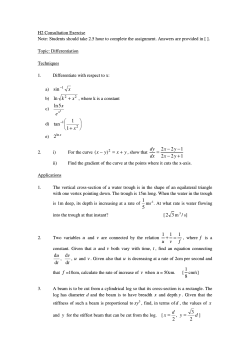
The point (0,−1) is never taken.
Figure 1: Missing Points.
Observe that as u varies, a circle is traced at the ‘height’ z = v. Another example is the sphere
given implicitly as X 2 + Y 2 + Z 2 − 1 = 0, and given parametrically by:
(
2u
2v 1 − u2 1 − v 2
2v
,
,
)
1 + v 2 1 + u2 1 + v 2 1 + u2 1 + v 2
One may check that:
x2 (u, v) + y 2 (u, v) + z 2 (u, v) = (
2v 2
) + z 2 (u, v) = 1
1 + v2
We make three remarks which we will clarify later. Firstly, not all implicitly defines curves have
a parametrization; in fact, most dont. One example is the the elliptic curve Y 2 = X(X 2 − 1).
However, every parametrically defined curve has an implict form, and similarly for parametrically
defined surfaces. This is proved by the method of resultants, a technique for eliminating variables.
Secondly, even when a parametrization exists, it may not cover the whole curve. Eor example,
for the parametrization c(t) of the circle above, we may tabulate points on the circle for various
values of t as below:
t
−2
−1
0
1
2
p(t) (− 45 , − 35 ) (−1, 0) (0, 1) (1, 0) ( 54 , − 35 )
We see that as t ranges over R, the point (0, −1) is never taken, and therefore is missing from the
image of the parametrization c(t). This is to be expected since the line is ‘open’ and the circle is a
‘closed’ curve. Similarly, for the cylinder, the points (0, −1, z) is never taken for any z: this simply
follows from the circle case above. For the sphere, we see that the point (0, 0, 1) is never taken by
the parametrization.
The third remark is that different approaches to the representation of curves and surfaces
serve different needs. For example, when in implicit form, it is difficult to produce points on the
curve/surface, for that means solving equations in one/two variables. On the other hand, the
parametrized representation makes it very convenient to produce points. On the other hand, given
a candidate point p, it is easy to check if p lies on the curve; one just have to check if p satisfies the
defining equations. Note that this question is hard to resolve for a parametrized curve.
2
Faces and Edges
Imagine, for the moment that we wish to represent parametrically, the whole circle. Since we have
seen as above, that the natrural parametrization fails; in fact no such parametrization exists, we
2
e1
start(e1)=
end(e4)
e2
e3
e4
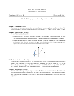
Figure 2: A Loop.
must reconcile with this fact, and at the same time, do get every point on the circle. One option
is to break the circle into two parts, and represent each part with a parametrization. Thus, for
example, the map c, restricted to [−1, 1] gives the ‘top’ half of the circle. The bottom half may be
t2 −1
represented by the parametrization d(t) = ( t22t
+1 , t2 +1 ). Note that d(t) was obtained by replacing t
by 1t in c(t). Thus t goes from 1 to −1, d(t) will trace the bottom half of the circle. Thus we may
represent the circle in terms of two parametrizations c, d : R → R2 , however, the domains of c, d are
restricted to the intervals [−1, +1].
2.1
Edges and Loops
Let us now define the entity edge as a pair (I, f ), where f is a function f : R → Rn , and I ⊂ R is an
oriented interval [a, b]. The edge may be identified as starting from the vertex f (a) and ending
at the vertex f (b) while tracing out f (t) for every point t between a and b. Note that ([a, b], f ) and
([b, a], f ), while geometrically being the same edge, are oriented inopposing directions. Thus the
orientation gives a direction to the edge, and this frequently very useful. The vertices f (a) and f (b)
will be denoted as start(e) and end(e). Typical kernels require the edge to not self-intersect and
that start(e) 6= end(e).
We thus see that our circle may be represented as two edges e1 = ([−1, 1], c(t)) and e2 =
([1, −1], d(t)). Also note that the orientation of e2 as going from 1 to −1 is convenient, as it ‘follows’
the orientation of e1 .
The arrangement above is a special case of a loop which is defined as a collection of edges
(e1 , e2 , . . . , ek ) where each ei is an edge, and start(ei ) = end(ei−1 ) with start(e1 ) = end(ek ). As
before, there are other geometric requirements for a loop which are implemented differently for
different kernels. One typical requirement is that no two edges ei and ej intersect other than the
case when i = j ± 1, then too only at the appropriate end-points.
2.2
Domains and Faces
A loop in the plane R2 always splits R2 into two parts, the inner (bounded) part and the outer
(unbounded) part. The orientation of the loop may be used select one of these two sub-parts. A
loop is said to be anti-clock-wise if there is a point in the bounded part such that the loops winds
around this point in an anti-clock-wise manner. Otherwise, the loop is called clockwise. The loop
in Figure 2 above is clock-wise.
Our next entity is the domain D which is a subset of R2 . The simplest domain D = domain(O)
is defined by a single loop O in the plane. If O is clockwise, then D is taken to be the unbounded
3
Outer Loop
I2
I1
Inner Loops
I1
I2
D
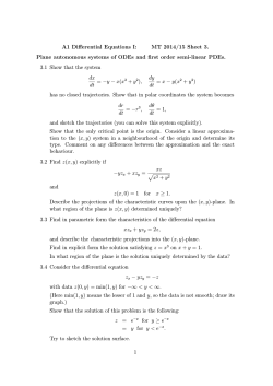
Figure 3: A Domain.
part outside (and including) the loop. If O is anti-clock-wise then D will denote the part inside (and
including) the loop. The general domain is the intersection of simple domains
D = domain(O1 ) ∩ domain(O2 ) ∩ . . . ∩ domain(Ok )
One may check that it suffices to require that O1 , . . . , Ok do not intersect, and that atmost one, say
O1 is oriented anti-clockwise, and others must be oriented clockwise. If D is bounded, then there
is indeed the O1 which is anti-clockwise. This loop is called the outer-loop, and the others are
called inner loops. Since, we will usually be interested in bounded domain, we will assume that D
is given by a list (L1 , . . . , Lk ) of mutually non-intersecting loops such that L1 is the outer-loop and
all other loops are inner.
A face may now be defined a tuple F = (D, f ) where f : R2 → R3 is a function, and D is a
domain. The points of the face are assume to come by restricting f to D. Thus, for all (u, v) ∈ D,
f (u, v) ∈ F . Various kernels require many other properties such as (i) F should not self-intersect,
(ii) f should be smooth, and so on.
We must add that the entities edge and face are geometric entities, since they must be accompanied by functions which actually do the parametrization. In contrast, the entities such as loop
and domain are topological or combinatorial since they are defined by a collection of geometric
entities in special configuration. Note that every edge e which occurs in one of the loops O defining
domain D, are plane edges, i.e., in R2 . Thus e = (I, g) where I is an oriented interval and g : R → R2
is the parametrization. Thus the composition g ◦ f is a map from R to R3 . This may be used to
define the co-edge e′ as the composition e′ = (I, g ◦ f ). This e′ is a space edge and defines a part
of the boundary of the face F . The space R3 is called the object space, while R2 , when it is used
to define the domain, is called the parametrization space.
Thus the data for a face includes (i) the domain, and the parametrizing function. The definition
for the domain will include its loops, each loop, its edges and co-edges and so on. Note that each
co-edge has an ‘owner’, viz., the face from which its definition came. The general solid is represented
as a collection of faces with certain co-edges identified. Thus, when face F1 meets face F2 along
an edge e, then the corresponding co-edges e1 (coming from F1 ) and e2 (from F2 ) are identified as
equal.
3
Polynomials and Resultants
C will stand for the field of complex numbers. Let t be a ‘variable’ and let R[t] (or C[t]) denote
the collection of all polynomials in the variable t with real (or complex) coefficients. The typical
4
Face F=(D,f)
edge e
f
Domain
D
Underlying
Surface
1111111111111111
0000000000000000
0000000000000000
1111111111111111
0000000000000000
1111111111111111
0000000000000000
1111111111111111
0000000000000000
1111111111111111
0000000000000000
1111111111111111
0000000000000000
1111111111111111
0000000000000000
1111111111111111
0000000000000000
1111111111111111
0000000000000000
1111111111111111
0000000000000000
1111111111111111
0000000000000000
1111111111111111
0000000000000000
1111111111111111
0000000000000000
1111111111111111
0000000000000000
1111111111111111
0000000000000000
1111111111111111
0000000000000000
1111111111111111
0000000000000000
1111111111111111
0000000000000000
1111111111111111
0000000000000000
1111111111111111
0000000000000000
1111111111111111
0000000000000000
1111111111111111
0000000000000000
1111111111111111
0000000000000000
1111111111111111
0000000000000000
1111111111111111
0000000000000000
1111111111111111
Co−edge e’
Figure 4: A Face.
polynomial p(t) is represented as
p(t) = ad td + ad−1 td−1 + . . . + a1 t1 + a0 t0
Let 1 ≤ m ≤ d be the largest number such that am 6= 0. The
m is called
degree of the
P the
Pinteger
i
i
b
t
may
a
t
and
q
=
polynomial
and
is
denoted
by
deg(p).
Two
polynomials
p
=
i
i
i
i
Pbe added:
P
if r = i ci ti = p + q, then ci = ai + bi for all i. Polynomials may be multiplied: if s = i di ti and
Pk
s = pq, then si = j=0 aj bi−j . Thus for example, d0 = a0 b0 , d1 = a0 b1 + a1 b0 , and so on. Note
that deg(pq) = deg(p) + deg(q), while deg(p + q) ≤ max(deg(p), deg(q)).
Let Vd denote the space of all polynomials p such that deg(p) ≤ d. The space Vd is a vector space
under polynomial addition. The dimension of Vd is d + 1 and {1, t, t2 , . . . , td } is an obvious basis of
Vd
We say that p divides
q if there P
is a polynomial r such that q = pr. We say that α ∈ C (or R)
P
is a root of p(t) = i ai ti if p(α) = i ai αi = 0.
Theorem 3.1 The division algorithm: Given polynomials a, b, there are unique polynomials q, r
such that a = bq + r, such that either r = 0 or deg(r) < deg(b).
Proof: The existence of q, r is the so-called long division algorithm. The uniqueness is easy too: if
a = bq + r = bq ′ + r, then b(q − q ′ ) = (r′ − r), whence, either q-q’=0, whence r′ − r = 0 as well, or
we have deg(b(q − q ′ )) ≥ deg(b), while deg(r′ − r) < deg(b), a contradiction. ✷
Corollary 3.2 If α is a root of polynomial p, then (t − α) divides p.
The following is a rewording of the famous fundamental theorem of algebra:
Theorem 3.3 Every polynomial p = ad td + . . . + a0 of degree d with real/complex coefficients may
Qk
be factorized over complex numbers as p(t) = ad i=1 (t − αi )mi , where the αi ’s are all distinct. This
factorization of p is unique, and the collection {α1 , . . . , αk } is the set of all roots of p. Furthermore,
m1 + . . . + mk = d, and the number mi is called the multiplicity of the root αi . If p has real
coefficients and α is a root of p with multiplicity m, then so is the complex conjugate α, and with
the same multiplicity.
We now come to an important result. Let p = am tm + . . . + a0 and q = bn tn + . . . + b0 be
two polynomials of degree m and n respectively. We ask if p and q have a common root. The
naive of doing this would be to solve p and q and then compare the roots of the two polynomials.
However, other than numerical solution, there is no known procedure to write down the roots of a
5
polynomials, given by its coefficients. It turns out that to check if p and q have a common root, it
does not quite require us to find the roots. This is by the famous gcd algorithm for polynomials.
Thus the gcd(p, q) is 1 (or equivalently, a non-zero constant) iff p and q do not have a common root.
Since the gcd is computable using the long-division process, it may be directly used to implicitize
parametric definitions of curves and surfaces. Consider, for example, the circle parametrized by
2t
1−t2
x = 1+t
2 and y = 1+t2 , or equivalently we have the polynomials p(x, y, t) and q(x, y, t) below:
xt2 − 2t + x = 0
(y + 1)t2 + (y − 1) = 0
Clearly, those points (x0 , y0 ) lie on the circle for which there is a t0 which is a common solution to
both the equations. In other words, the condition that p0 (t) = p(x0 , y0 , t) and q0 (t) = q(x0 , y0 , t)
have a common solution is that their gcd(p0 (t), q0 (t)) should have the zero constant term. The gcd
can be computed by the long-division algorithm: dividing p0 by q0 , we get the remainder as:
−2t +
Dividing q0 by the remainder, we get:
2x0
y0 + 1
x20 + y02 − 1
y+1
Thus, the gcd has zero constant term tells us that the numerator must be zero, which gives us the
implicit equation of the circle, and the denominator y + 1 gives us the exceptional point (0, −1),
with y + 1 = 0.
In general, this process can be used to eliminate any variable from two equations. A more explicit
formulation is that of the resultant. We have:
Proposition 3.4 If the degrees of p and q are m and n respectively, then gcd(p, q) 6= 1 if and only
if there are polynomials f and g such that pf = qg and deg(pf ) < m + n.
Proof: Suppose that (t − α) was a common root. Then p = (t − α)p′ and q = (t − α)q ′ . Thus with
f = q ′ and g = q ′ , we have pq ′ = qp′ = (t − α)p′ q ′ . Also note that deg(pq ′ ) = m + n − 1 < m + n.
Conversely, if there were f, g as above, and assuming that p and q have no roots in common, for
every root α of p with multiplicity m, we see that (t − α)m divides pf , the LHS, and therefore must
divide the RHS, qg. Since α is not a root of q, we must have that (t − α)m must divide g. In other
words, deg(g) ≥ m and deg(qg) ≥ m + n, a contradiction. ✷
We know show that the condition of proposition 3.4 is easily checkable. We construct the polynomials pi = ti p, for i = 0, 1, . . . , n − 1, and q j = tj q, where j = 0, 1, . . . , m − 1. Let P = {p0 , . . . , pn−1 }
and Q = {q 0 , . . . , q m−1 } and note that every polynomial of P ∪ Q is of degree atmost m + n − 1.
Thus the set P ∪ Q is potentially a collection of m + n polynomials in the vector space Vm+n−1 , the
space of polynomials of degree atmost m + n − 1. We now have the following proposition:
Proposition 3.5 The polynomials p and q have a common root if and only if the polynomials in
P ∪ Q are linearly dependent.
P
P
Proof: Let α0 , . . . , αn−1 and β0 , . . . , βm−1 be numbers, not all zero, such that i αi pi + j βj q j = 0
(inside Vm+n−1 ). We thus see that:
(α0 t0 + . . . + αn−1 tn−1 )p = (−β0 t0 + . . . + βm−1 tm−1 )q
6
P
P
In other words, with i αi ti as f and i (−βi )ti as g, we have pf = qg is a polynomial of degree
not exceeding than m + n − 1. Conversely, if we have f and g as above, then they can be unfolded
to construct α’s and β’s, a linear dependence between the polynomials in P ∪ Q. ✷.
For the polynomials p and q as above, we define the resultant matrix Rest (p, q) (with the t to
denote the variable) as the (m + n) × (m + n) matrix below:


am am−1
...
a0
0
0
... 0
 0
am
am−1 . . . a0
0
... 0 




..
..
 0
.
...
.
... 


 0
...
0
0 am am−1 . . . a0 


Rest (p, q) = 
...
b0
0
0
... 0 

 bn bn−1
 0
bn
bn−1 . . . b0
0
... 0 




..
..
 0
.
...
.
... 
0
...
0
0
bn
bn−1
...
b0
Proposition 3.6 The polynomials p and q have a common root iff det(Rest (p, q)) = 0, or in other
words, if the resultant matrix is singular.
Proof: Recall that a basis of Vm+n−1 are the polynomials {t0 , t1 , . . . , tm+n−1 }. Whence, any polynomial in Vm+n−1 may be expressed as a linear combination in this basis. In particular, we see that
ordering the elements of P ∪ Q as {pn−1 , . . . , p1 , p0 , q m−1 , . . . , q 1 , q 0 }, we see that:

 n−1  
am am−1
...
a0
0
0
... 0
p

..   0
am
am−1 . . . a0
0
... 0 

  m+n−1 

. 


 t

.
.
..
.
 p1   0
...
.
... 
tm+n−2 






 p0   0
.
.
.
0
0
a
a
.
.
.
a


..
m
m−1
0

 m−1  = 

.
  bn bn−1

 q
.
.
.
b
0
0
.
.
.
0

0
 


1

t
  0


.
b
b
.
.
.
b
0
.
.
.
0
n
n−1
0
.



. 
t0
 


.
.
..
..
 q1   0
...
... 
0
...
0
0 bn bn−1 . . . b0
10
Thus, P ∪ Q are linearly dependent iff Rest (p, q) is singular. ✷
We will illustrate a few application of the above proposition. Consider the case when p = t2 −4t+3
and q = −t2 − 1. To check if they share a root, we form the resultant matrix:


1 −4 3
0
 0 1 −4 3 

R=
 1 0 −1 0 
0 1
0 −1
We see that det(R) = 0 and that p, q above indeed share the root t = 1.
Another interesting case is to check if the general polynomial f (t) = at2 + bt + c has a double
root. This is equivalent to checking if f and f ′ , the derivative of f w.r.t. t have a common root.
Clearly f ′ = 2at + b, and thus the resultant is:


a
b c
D =  2a b 0 
0 2a b
7
One may check that det(D) = −a(b2 − 4ac). Since a 6= 0, we see that f hasa double root if the
discriminant b2 − 4ac = 0. The general discriminant of a polynomial f is defined to be Rest (f, f ′ ).
We now apply this technique to convert parametric represnetations of a curve to implicit ones.
2t
1−t2
We do this by an example, the general case will be left to the reader. Recall that c(t) = ( 1+t
2 , 1+t2 )
was the parametrization of the circle. Thus, for an (x, y), it would lie on the circle iff the equations
1−t2
2t
x = 1+t
2 and y = 1+t2 have a common root. Clearing denominators, we have:
xt2 − 2t + x
=
(1 + y)t2 + y − 1 =
0
0
Forming the resultant of the above equations, we have:

x
−2
x
0
 0
x
−2
x
S=
 1+y
0
y−1
0
0
1+y
0
y−1




Expanding det(S) we get 4(x2 + y 2 − 1), which is the required implicit form for the circle.
4
Polynomial Bases
Polynomials will serve as the central object in which functions will be specified. The main advantage
being their familiarity, ease in representation and implementation of operations, and finally, the
strength of various theorems such as the Weierstrass Approximation theorem.
Our first study will be that of polynomials in one variable, i.e., the space R[t]. Recall that Vd
is the d + 1-dimensional subspace of polynomials of degree d or less. The standard basis for Vd is
obviously, T = {1, t, t2 , . . . , td }. Different bases of Vd have different practical uses. For example, if
we were given f : R → R, and the values f (0), f ′ (0), . . . , f d (0). For this data, a good approximation
to f would be
d
X
f i (0) k
f (t) ≈ T (f ) =
t
i!
i=0
Thus we see that the basis T is suited for the purpose of approximating f by its derivatives at 0.
Of course, if t = 1 were to be special, then the basis T1 = {1, t − 1, (t − 1)2 , . . . , (t − 1)d } would do
the job.
The general interpolation problem is given by (i) a procedure to conduct d + 1 independent
observations of the function f , (ii) the construction of a basis P = {p0 , . . . , pd } of Vd , which is
specially suited to the nature of the observations, and (iii) the observations o0 (f ), . . . , od (f ) and the
Pd
interpolant P (f ) = i=0 oi (f )pi . Note that the basis T depends only on (i) and not on the function
f to be approximated/interpolated. Also note that the basis T above fits the above paradigm.
Let Λ = {λ0 , . . . , λd } be a fixed collection of distinct real/complex numbers. Another important
basis of Vd is the Lagrange basis, L(λ0 , . . . , λd ). Let (i) above correspond to the observation of
f at the point λi , and thus oi (f ) = f (λi ). The lagrange basis L = {L0 , . . . , Ld } is such that
Pd
L(f )(t) = i=0 f (λi )Li (t) is a degree-d polynomial such that L(f )(λi ) = f (λi ). Just this requirment
forces us to have Li (λj ) = δij if i 6= j and 1 otherwise. One may solve for Li as follows: let
P
P
Li = j aij tj . Thus δij = Li (λj ) requires δij = j aij λji . This is easily expressed in matrix form
as:
8

1
 0



0
 
... 0
a00
 a10
... 0 
 
=
..
 
.
ad0
... 0 1
0
1
..
.
a01
a11
..
.
. . . a0d
. . . a1d
..
.
ad1
. . . add
λ00
  λ10



λd0

λ01
λ11
..
.
λd1

. . . λ0d
. . . λ1d 


..

.
d
. . . λd
Thus, we see that the lagrange basis may be expressed in terms of the standard basis by inverting
the Van der Monde matrix Λ = (λij ).
Both, the standard basis and the lagrange basis are special cases of the Hermite
basis: We are
P
given distinct points α0 , . . . , αk , and positive integers m0 , . . . , mk such that i mi = d + 1. The
observations are the first mi -th derivatives of f at the point αi . Thus, given f (α0 ), f ′ (α0 ) and so on
upto f m0 −1 (α0 ), and so on for other α’s, there is a unique polynomial H(f )(t) matching this data.
The basis for this is the Hermite basis for this data. Note that when α0 = 0, and m1 = d + 1, then
we get the standard basis, while on the other end, if we have k = d and mi = 1 for all i, then we
have the lagrange basis.
An even more general paradigm is the following: Let o0 , . . . , on be linear observations on the
space Vn . In other words, oi : Vn → R are functions such that oi (αp + q) = αoi (p) + oi (q), where
α ∈ R/C, and p, q ∈ Vn . Examples of such observations are of course, p → p(0) or p → p′ (0). Other
R1
Rb
interesting examples are p → 0 p(t)dt, or a t · p(t)dt. Note that all these ‘integral’ observations are
linear.
We would like to find polynomials p0 , . . . , pn such that oi (pj ) = 0 is i 6= j and 1 when i = j,
or simply oi (p
j ) = δij , the kronecker delta. We choose a standard basis, say Q = {q0 , . . . , qn }, and
P
express pi = j aij qj , or in matrix notation P (t) = AQ(t). Applying the observation oi , we have:
 
 
a00
δi,0
oi (p0 )
  ..   ..

..
= . = .

.
an0
δi,n
oi (pn )



oi (q0 )
a0n

..
..  

.
. 
oi (qn )
. . . ann
...
Combining this for all i, we write Λ = (oj (qi )) we have:
I = AΛ
Thus, there is such a basis iff Λ is invertible.
Coming back, let us assume that we have a function f : [0, 1] → R. Our first task is to approximate f in the prescribed interval within a given ǫ > 0. We have the famous:
Theorem 4.1 The Weierstrass Approximation Theorem: Given any continuous function f :
[0, 1] → R, and an ǫ > 0, we have a polynomial p such that for all t ∈ [0, 1], we have |f (t) − p(t)| < ǫ.
One may represent this pictorially in the figure below: The function f appears in bold. The
ǫ-envelope of the function f is also shown and the graph of the desired approximating polynomial p.
The basic question is about how to implement the WAT. Surely, the first attempt would be to use
n−1 n
the lagrange basis. In other words, let us select Λn = { n0 , 1,n
, . . . , n , n }, the n + 1 points equally
spaced inP
the interval [0, 1]. Given the function f , let yi = f ( ni ), and form the lagrange interpolant
Ln (f ) = i yi Li (t). We note that, while Ln (f ) matches f exactly on the points Λn , it strays very
far from f in the interim. One suggestion then would be to increase n, but we see that the situation
actually gets worse. As n increases, the n-th interpolant may actually worsen, and stay out of the
ǫ-envelope for most points of the interval.
9
Function f
Upper
Envelope
Lower
Polynomial p
Figure 5: The Weierstrass Approximation Theorem (WAT).
00
11
11111111
00000000
00
11
00000000
11111111
function f
00000000
11111111
00000000
11111111
00000000
11111111
00000000
11111111
00000000
11111111
0111111111
00000000
00000000
11111111
00000000
11111111
00000000
11111111
0000000011111111
11111111
00
11
00000000
11111111
00000000
00000000
11111111
00
11
00000000
11111111
00000000
11111111
0000000011111111
11111111
00000000
11111111
00000000
00000000
11111111
00000000
11111111
00000000
11111111
00000000
11111111
00000000
0000000011111111
0000000011111111
11111111
00000000
11111111
11
00
00000000
11111111
00000000
11111111
00000000
11111111
00000000
11111111
00000000
11111111
00000000
11111111
00000000
11111111
0000000011111111
0000000011111111
00000000
0000000011111111
11111111
2/4
3/4
Approximation S(f)
0/3
1/4
1/3
2/3
3/3
Figure 6: The Sohoni Approximation Theorem (SAT)!
Here is a simple basis, which though not polynomial, atleast approximates continuous. For a
i
i+1
chosen n, let pi = ni , and let Ii be the interval [ n+1
, n+1
]. Let χi be the function which is 0 outside
Ii and 1 inside. In other words, χi (t) = 1 if t ∈ Ii . Consider s = {χ0 , . . . , χn } as a collection of n + 1
functions on the interval [0, 1]. For a given P
function f : [0, 1] → R, we observe the function f at the
n
points f (pi ) and for the function S n (f ) = i=0 f (pi )χi . The case n = 3 is indicated in the Figure
6. Note that pi ∈ Ii and thus S n (f ) agrees with f at some point in every interval Ii .
We have the famous Sohoni Approximation Theorem:
Theorem 4.2 For any continuous f : [0, 1] → R, and an ǫ > 0, there is an N such that for all
n > N , S n (f ) approximates f to within ǫ. In other words, |S n (f )(t) − f (t)| < ǫ for all t ∈ [0, 1].
The proof of this is straight-forward and is omitted here.
Of course, this basis is of very limited use since it is not polynomial, not continuous and so on.
But the point was that each χi had support only within Ii and thus a scalar multiple of χi could be
chosen to approximate f in Ii . The larger the n, the finer is the approximation. Thus, if we could
find polynomials with similar properties, we would have an implementable version of WAT. This
need is satisfied precisely
by the Bernstein basis.
Let Bin (t) = ni ti (1 − t)n−i , regarded as a function on the interval [0, 1]. Let B n = {B0n , . . . , Bnn }:
this collection is called the Bernstein basis. Note that each Bin (t) is a polynomial of degree atmost
n. We now state some properties of the collection B n .
10
Lemma 4.3
1. B n is a basis of Vn .
2. Bin (t) ≥ 0 for all t ∈ [0, 1]. Furthermore,
3.
dBin (t)
dt
n−1
= n(Bi−1
(t) − Bin−1 (t)).
R1
0
Bin (t)dt =
1
n+1 .
4. The maximum value of Bin (t) in the interval [0, 1] occurs at the point
i
n.
Proof:
1. The first part is easy: If we express Bin (t) in terms of the basis {1, t, t2 , . . . , tn } we see that
n i
Bin (t) =
t + higher terms
i
Thus the matrix expressing B n in terms of the standard basis is upper triangular with non-zero
entries on the diagonal, and therefore is invertible. This proves that B n is a basis.
2. Clearly, for t ∈ [0, 1], both t and (1 − t) are non-negative. The second part follows a simple
induction:
Z 1
Z 1 n i
n
t (1 − t)n−i dt
Bi (t)dt =
i
0
0
i+1
Z
n n − i 1 i+1
n t
(1 − t)n−i +
=
t (1 − t)n−i−1 dt
i i+1 0
i i+1
Z 1
1
n+1
n
Bi+1
(t)|10 +
Bi+1
(t)dt
=
n+1
0
This is easily settled to get the result.
3. This is easily shown, and we move to (4). Solving for
0
dBin (t)
dt
= 0, gives us
n−1
= Bi−1
(t) − Bin−1 (t)
t
1−t
−
=
n−i i
= i − nt
The result follows. ✷
We thus see that the bernstein basis has properties similar to the basis S n . In fact, we have
the
theorem of Bernstein: For a fixed continuous f : [0, 1] → R, and an n, let B n (f )(t) =
Pn famous
i
n
n
i=0 f ( n )Bi (t). Note that B (f )(t) is a polynomial of degree n and is obtained as a linear combination of the bernstein polynomials. Furthermore, the coefficient of Bin (t) is precisely the observation
f ( ni ), as in the SAT. We have:
Theorem 4.4 For any continuous f : [0, 1] → R, and an ǫ > 0, there is an N such that for all
n > N , B n (f ) approximates f to within ǫ. In other words, |B n (f )(t) − f (t)| < ǫ for all t ∈ [0, 1].
11
3
B33
B0
3
B23
B1
0
1
Figure 7: The Bernstein Polynomials for n = 3
The proof of this theorem is rather intricate, and we shall skip it. However, we note that
B n (f )(0) =
n
X
i
f ( )Bin (0)
n
i=0
Since Bin (0) = 0 unless i = 0, and then it is 1, we have that B n (f )(0) = f (0). Similarly, we have
B n (f )(1) = f (1), and thus the approximation B n (f ) interpolates f at 0 and 1. However, this not
the case at the intermediate points; in this it differs from the lagrange basis.
Interestingly, we also note that
(B n (f ))′ (0) =
X
i
i
n−1
(0) − Bin−1 (0))
f ( ) · n · (Bi−1
n
The only terms which matter are i = 0 and i = 1, and we have:
1
f (1/n) − f (0)
(B n (f ))′ (0) = n(f ( ) − f (0)) =
n
1/n
5
Bezier Curves
We now move to the problem of constructing edges in R2 or R3 . Bezier was a frenchman working
in a car design shop, and was one of the first persons to use the Bernstein basis for edge and face
design. the basic object in the design and analysis of bezier curves is the control-point sequence,
which is also known as the control polygon.
Suppose that we have a curve C, as shown in figure 8, which is available to us as drawn by an
artist. Our task is to parametrize this curve C. The first step is to fix the start vertex and the endvertex. Having done this, let us assume that we desire to parametrize it with the interval [0, 1]. Next,
we imagine a cyclist travelling along the curve, starting at t = 0 from the start vertex, and arriving at
the end vertex at time t = 1. As the cyclist moves, we construct the functions x(t), y(t) : [0, 1] → R,
which read out the x and the y-coordinate of the cyclist with time. Having plotted these associated
functions x(t), y(t), we may now use the bernstein basis for their approximation.
For example, we choose an n (n = 3 in figure 8), and proceed to construct
the vectors pi =
Pn
[x(i/n), y(i/n)] for i = 0, . . . , n. The bezier curve P n (C)(t) is defined as i=0 pi Bin (t). Note that
P n (C) evaluates to a linear combination of the vectors p0 , . . . , pn , whose coefficients chane with t.
12
2.5
Z
2
1.5
1
1.8
2.5
1.6
1.4
2
1.2
1.5
1
Y
1
X
Figure 8: A curve C and its approximate parametrization.
p1
p3
p2
p1
p0
p0
p2
p2
p3
p1
p0
p0
p1
p3
p3
p2
Figure 9: Examples of Control Polygons and their curves, for n = 3
Indeed, the function P n (C) is obtained by the simulteneous approximation of x(t) and y(t) by the
bernstein recipe above.
It is possible that P n (C) does fails to be close enough to C and n need to be hiked up. See, in the
figure, that P 6 (C) approximates C better than P 3 (C). In any case, note that since B n (x)(0) = x(0)
and B n (y)(0) = y(0), we have P n (C)(0) = C(0), the start vertex, and similarly at t = 1.
The vector coefficients, p0 , . . . , pn , in that order is called the control polygon. The polygon
determines the approximating curve P n completely. While we have been chosing the control points
to lie on the curve to be approximated, that is not really required. Frequently, the control points
may be chosen outside the curve, and yet P n (t) hugs C better.
Examples of a few control polygons and the approximating curves are shown in figure 9.
Thus, we have arrived at the bezier representation of a curve, which is parametrized by the
degree n, and a sequence P = [p0 , . . . , pn ] called the control polygon. The curve may be equivalently
stored as the tuple (n, P ), which is a fairly compact representation of the parametrization. The
evaluatePof C(t) may be done by computing the coefficients Bin (t) and forming the linear combination
C(t) = i pi Bin (t). We have also seen that the above curve interpolates the first and the last control
13
point. The derivative C ′ (t) is also easily caluclated:
C ′ (t)
=
X
pi
i
=
=
X
i
n−1
X
i=0
dBin (t)
dt
n−1
pi · n · (Bi−1
(t) − Bin−1 (t))
n · (pi+1 − pi )Bin−1 (t)
Thus, C ′ (t) can be easily written in Bezier form as (n − 1, P ′ ) where, P ′ = [p1 − p0 , p2 − p1 , . . . , pn −
pn−1 ]. In general, the k-th derivative is also easily expressed as
C k (t)
n−k
k
XX
n!
k
pi+j Bin−k (t)
(−1)k−j
j
(n − k)! i=0 j=0
=
(1)
We also note here that geometric transformations on the curve are easily implemented by effecting
the same transformation on the control points. Let P = [p0 , . . . , pn ] be the 3 × (n + 1) matrix
representing the control points of a space curve. The general point is given by the equation:
 n

B0 (t)


..
C(t) = [p0 , . . . pn ] 

.
Bnn (t)
we abbreviate this to C(t) = P B(t). Thus is A is a linear transformation of the curve, say C(t) →
AC(t), where A is a 3 × 3-matrix, then AC(t) = AP B(t). Thus, the operator A operates on P from
the left and B(t) from the right, and they commute. Thus whether we evaluate the curve first and
then operate on it, or operate on the control points and then evaluate the curve, we get the same
answer. Thus, to store the transformed curve, we may as well store just the transformed control
points. Another example of this is translation. say, we wish to translate the curve by a fixed vector
v ∈ R3 . In other words, let D(t) = C(t) + v. We put Q = [p0 + v, . . . , pn + v], and observe that
QB(t) = P B(t) + [v, v, . . . , v]B(t)
Now, note that
X
i
Thus,
Bin (t)
X n
=
ti (1 − t)n−i = (1 − t + t)n = 1
i
i
X
i
v·
Bin (t)
X n
ti = v
=v·
i
i
Thus QB(t) = C(t) + v, and D(t) is thus represented merely by translating the control points by v.
6
Degree Elevation and Subdivision
Frequently, it is required to represent a given parametric curve C = (n, P ) by a higher degree curve.
This need arises when the current degree of representation is deemed inadequate. Since an elevation
14
11
00
q2
p0=q0
11
00
11
00
q1
p2
q3
11
00
1 0
0
1
p1
0/3
0110 p3=q4
2/4
1/4
1/3
3/4
3/3
2/3
Figure 10: Degree elevation from n = 3 to n = 4.
of the degree by one, gives an additional control point, it may be desirable to elevate the degree
of C. In other words, we would like to compute the control polygon Q = [q0 , . . . , qn+1 ] so that
C = [n, P ] = [n + 1, Q].
For the standard basis, viz., T n = {1, t, . . . , tn }, we see that T n ⊆ T n+1 , and thus a polynomial
expressed in tn is automatically expressed in the higher degree basis T n+1 . In other words, in the
standard basis Q = [p0 , . . . , pn , 0]. This is not the case for the bernstein basis, since Bin 6∈ B n+1 .
However, we see that:
Bin (t)
= (1 − t + t) · Bin (t)
n i
= ((1 − t) + t)
t (1 − t)n−i
i
n i
n i+1
n−i+1
=
t (1 − t)
+
t (1 − t)n−i
i
i
i + 1 n+1
n − i + 1 n+1
Bi (t) +
B
(t)
=
n+1
n + 1 i+1
Thus we have that
n
X
pi Bin
=
n
X
pi (
i=0
i=0
=
n+1
X
(
i=0
n − i + 1 n+1
i + 1 n+1
Bi (t) +
B
(t))
n+1
n + 1 i+1
i
n−i+1
pi−1 +
pi+1 )Bin+1 (t)
n+1
n+1
i
Thus we see that qi = n+1
pi−1 + n−i+1
n+1 pi+1 . This is pictorially seen much better in figure 10. The new
1
n+1
0
, n+1
, . . . , n+1
},
control ponts are obtained by interpolating the control polygon at the points { n+1
in that order.
At this point, we turn to the implementation of the evaluation of a point on a typical bezier
curve for a given parameter value, sayP
t. The naive algorithm would compute each Bin (t), and then
n
form the linear combination P (t) =
i Bi (t)pi . A clever way of organising the computation is
given by the de-Casteljeu algorithm. This scheme, besides being efficient and numerically stable, is
also an important geometric formalism. The scheme is best illustrated by the following Figure 11.
The scheme creates the variables p[i,j], with i ≤ j. The variables p[i,i] are instantiated to the
control point pi . The main iteration is the following:
15
p[0]
p[1]
t
1−t
p[2]
t
1−t
p[0,1]
p[3]
1−t
p[1,2]
t
1−t
t
p[2,3]
t
1−t
p[0,2]
p[1,3]
t
1−t
p[0,3]
Figure 11: The de Casteljeu scheme for n = 3
P[2,2]
P[1,2]
P[1,1]
P[1,3]
P[2,3]
P[0,3]
P[0,1]
P[0,2]
P[0,0]
t=1/4
P[3,3]
Figure 12: The geometry of the de Casteljeu scheme for n = 3
P[i,j+1]=(1-t)P[i,j]+tP[i+1,j+1].
It is easy to see that the iteration actually works, and this is best seen from the schema in Figure
11. In the figure, the arrows have been marked with the multipliers t or (1 − t). Note that every right
arrow has a (1 − t) and every left arrow, a t. The coefficient of p[i,i] in p[0,n] is parametrized
by the number of paths from p[i,i] to p[0,n]. Since, anysuch path will have exactly i left-arrows
and (n − i) right-arrows, we see that there are exactly ni such paths, and each has a multiplier
ti (1 − t)n−i . Thus p[i,i] appears with the coefficient Bin (t), as required.
The geometric significance of the de Casteljeu algorithm is also nice, and is illustrated in Figure
12. In that figure, we show the the points p[i,j] for n = 3. Every succesive point is obtained as a
convex combination of points in the previous layer. The final point p[0,3] is taken to lie on the
curve. This also proves that the final point is a convex combination of convex combinations etc., of
the control points, and thus sits inside the convex hull of the control polygon.
Another point which we note now, and we will use later is that, is clear from the schema of the
de Casteljeu algorithm. For a fixed t, the points p[0,j] may be expressed as
p[0, j] =
j
X
pi Bij (t)
i=0
The second operation which we wish to analyse is called subdivision. Let e = ([0, 1], f ) be an
edge, with f : R → R3 . For a 0 < c < 1, we wish to construct the edge e′ which corresponds to the
16
segment [0, c] of e, however, we wish to re-parametrize it as from [0, 1]. In other words, we wish to
compute g such that g(t) = f (ct) for t ∈ [0, 1].
P
P
Again, in the standard basis, this is easy: if f (t) = i pi ti , then f (ct) = i (ci pi )ti . Thus, with
Q = [c0 p0 , . . . , cn pn ], we have that Q parametrizes the ‘subdivided’ curve g in the standard basis.
We P
compute this g when f is given as a bezier curve,
P (n, P = [p0 , . . . , pn ]). In other words, let
f (t) = i Bin (t)pi , we find Q = [q0 , . . . , qn ] such that i qi Bin (t) = f (ct).
The basic calculation is to express Bin (ct) in terms of {Bjn (t)|j = 0, . . . , n} and we begin in
earnest:
n
n i i
(ct)i (1 − ct)n−i =
c t {(1 − c)t + (1 − t)}n−i
i
i
n−i X
n
i i
=
c (1 − c)k ti+k (1 − t)n−i−k
i
k
k=0
n−i X
n
i+k
n−i−k i + k
ci (1 − c)k
t (1 − t)
=
i
i+k
k=0
=
n−i
X
n
Bi+k
(t)Bii+k (c)
k=0
With this small calculation behind us, we apply the usual trick of interchanging summations, and
see that:
X
pi Bin (ct)
=
=
X
pi
i
i
=
X
i
=
n
X
j=0
n−i
X
n
Bi+k
(t)Bii+k (c)
k=0
pi
X
Bjn (t)Bij (c)
i≤j≤n
Bjn (t)
j
X
pi Bij (c)
i=0
Pj
Now, we recall that i=0 pi Bij (c) is precisely p[0,j], a quantity which is computed during the
computation of the point f (c) = P (c). Thus, for the curve g(t) = f (ct), the control point sequence
is [p[0, 0](c), p[0, 1](c), . . . , p[0, n](c)]. This is pictorailly illustrated in Figure 13 below. Another
important point is that while the control point sequence QL = [p[0, 0](c), p[0, 1](c), . . . , p[0, n](c)]
parametrizes the curve CL for the interval [0, c], the sequence from the right, i.e., QR = [P [0, n](c), P [1, n](c), . . . , P [n, n]
parametrizes the curve CR in the interval [c, 1]. Since both CL and CR are part of the same curve
C, it must be that all derivatives of CL at it end-point equal those of CR at its start point. Thus
in the de Casteljeu triangle, if we start with a sequence of control points and fix a c, then the the
left hand side of the triangle and the right hand side of the triangle correspond to control points for
curves all of whose derivatives match.
k
In other words, we have that CLk (1) = CR
(0) for all k, whence, following Eqn. (1), we have the
relation:
k
k
X
X
k−j k
k−j k
p[0, j](c)
(2)
(−1)
p[n − k + j, n](c) =
(−1)
j
j
j=0
j=0
17
P[1]
c=3/4
P[0,1]
P[1,2]
P[0,2]
P[2]
P[0]
g(ct)
Control points: [P[0,0], P[0,1], P[0,2]]
Figure 13: The Subdivision Scheme
7
B-Splines
In this section we will develop the theory of B-Splines, or simply splines. These structures are
generalizations of bernstein/bezier systems, and overcome some of the drawbacks of the bezier
scheme. To name a few, if we wish to design a long curve with many contours, this would require
many control points, thus raising the degree of the bezier curve. The rise in the degree affects the
evaluation time (by the de Casteljeu algorithm) quadratically, which is expensive. Another irritation
is that local modifications of a few control points changes the curve everywhare. This is because
every bernstein polynomial is non-zero on the open interval (0, 1), An option is to split the curve into
many parts and design them separately. However, in this case, the derivatives have to be matched
at the end-points and this has to be done rather delicately.
7.1
B-Spline basics.
Splines are a device to the above systematically. Essentially, a spline is a continuous piece-wise
polynomial function with clearly specified cross-derivative matching. Let us fix the degree to say, n.
Let us have reals numbers a1 < a2 < . . . < ak and numbers m2 , . . . , mk−1 with each mi ≤ n. For a
polynomial p, we refer to its j-th derivative as pj .
Definition 7.1 A spline is a is a collection (p1 , . . . , pk−1 ) of polynomials of degree bounded by n
such that for all i = 2, . . . , k − 1, we have pi−1 (ai ) = pi (ai ), p1i−1 (ai ) = p1i (ai ), and so on till
n−mi
i
(ai ). the condition may be succintly expressed as:
pn−m
i−1 (ai ) = pi
pji−1 (ai ) = pi (ai ) f or i = 2, . . . , k − 1 and j = 0, 1, . . . , n − mi
In other words, we may define a function f : [a1 , ak ] → R such that f (t) = pi (t) when t ∈
[ai , ai+1 ]. The continuity requirements above ensure that f is continuous, and differentiable (n−mi )times at ai .
The data (a1 < . . . < ak ), and m1 , . . . , mk−1 is usually specified as a knot vector which we
describe now. For a fixed degree n, a knot vector is a sequence of reals α = (α1 ≤ α2 ≤ . . . ≤ αm )
with the following properties: (i) α1 = α2 = . . . = αn−1 , (ii) αm−n+1 = αm−n+2 = . . . = αm ,
and (iii), αi < αi+n−1 for i = 1, . . . , m − n, or in other words, other than the n duplications in
the beginning and the end, there is no sequence of n + 1 duplicates. the representation of the data
(a1 < a2 . . . < ak ) and m1 , . . . , mk−1 is the knot vector:
(a1 , . . . , a1 , a2 , . . . , ak−1 , ak−1 , . . . , ak , . . . , ak )
18
Here a1 and ak occur n times, while every other ai occurs mi−1 times. This may also be written as
Pk−1
mk−1 n
2
an1 am
2 . . . ak−1 ak . Note that
i=2 mi + 2n = m, the length of the knot vector.
Given a knot vector α, we define the space V (α) as the space of all spline function for the know
vector α. It is clear that this a vector space of functions, since if f1 , f2 ∈ V (α), then f1 + f2 will
have the same continuity properties that f1 and f2 share, and thus will belong to V (α).
Let us compute the dimension of this space. Clearly, since every element f ∈ V (α) is fiven by
a sequence of k − 1 polynomials, each of degree n, the maximum dimension of this vector space is
(k − 1)(n + 1). However, the continuity equations are many, indeed, for each ai , i = 2, . . . , k − 1,
there are n − mi + 1 of them. Thus we have the net dimension as:
(k − 1)(n + 1) −
k−1
X
i=2
(n − mi + 1) = 1 + n +
k−1
X
mi
i=2
In terms of m, we have dim(V (α)) = m − n + 1.
As an example, we see that the knot vector β = 0n 1n (of length 2n) corresponds to the familiar
space Vn of polynomials of degree n on [0, 1]. There are no side conditions, since k = 2. Thus
dim(V (β)) = m − n + 1 = n + 1.
Just as with the bernstein polynomials, the numbers {0/n, 1/n, . . . , n/n} were special, for they
corresponded to points in [0, 1] where observations {p0 , . . . , pn } could be made. The number of these
observations equalled the dimension n + 1 of Vn . Furthermore, the bernstein basis Bin was such that
these observations served as the coefficients of the approximating polynomial B n (P ). A similar
situation prevails for an arbitrary knot vector. The special set of points Ξ = {ξ1 , . . . , ξm−n+1 } are
called the Greville abscissa, and there are exactly m − n + 1 of them. There are the spline basis
functions Ni (α)(t) for the space V (α).
The ξi are easily defined:
αi + α2 + . . . + αi+n−1
ξi =
n
Thus the greville abscissa are “moving averages” of n consecutive knots. Note that since α1 = α2 =
. . . = αn , and similarly for the last knot, we have ξ1 = α1 , and ξm−n+1 = αm−n+1 . Also observe
that for β = 0n 1n , the moving averages are (0 + . . . 0 + 1 + . . . + 1)/n, and thus Ξ = {0/n, . . . , n/n}.
as in the bezier case, there is a sequence of observations P = (p1 , . . . , pm−n+1 ) called the control
polygon which form the schema for any element of V (α). See figure 14 for an example. The actual
spline function given by the coefficients P = [p1 , . . . , pmn +1 ] is given by:
N (P ) =
m−n+1
X
pi Ni (α)(t)
i=0
The basis functions Ni (α) are almost never used, but an evaluation strategy for any B-spline
function is given as an algorithm, very similar to de Casteljeu. Given the control polygon P , and the
parameter value t ∈ [α1 , αm ], there is a ‘triangular’ scheme to evaluate P (t), and we shall elaborate
that in the next subsection. That scheme depends on the basic subroutine of knot insertion, which
we now describe.
Given two knot vectors α and α′ , we say that α′ is obtained by inserting β into α, if the set
{α1 , . . . , αm } ∪ {β} arranged in ascending order is the knot vector α′ . In other words, there is an r
such that:
α′ = α1 , . . . , αr−1 , β, αr , . . . , αm
such that β < αr . let Ξ′ be the greville absiccas of α′ . Note that for i = 1, . . . , r − n, we have that
ξi′ = ξi , and that for j = r + 1, . . . , m − n + 2, we have ξj′ = ξj−1 . Furthermore, we see that for
19
p
p
p2
4
1
p
5
p
α
[0001222]
degree=3
3
ξ1=0
ξ2=1/3
ξ3=1
ξ 4=5/3
ξ5=2
Figure 14: A degree 3 B-spline control polygon and Greville abscissa.
j = r − n + 1, . . . , r, we have:
ξj−1 =
αj + . . . + αr−1 + β + αr + . . . + αj+n−2
αj−1 + αj + . . . + αj+n−2
≤=
= ξj′
n
n
αj + αj+1 + . . . + αj+n−1
αj + . . . + αr−1 + β + αr + . . . + αj+n−2
≤
= ξj
n
n
We further have:
ξj′ =
ξj′
=
αj+n−1 − β
β − αj−1
ξj−1 +
ξj
αj+n−1 − αj−1
αj+n−1 − αj−1
(3)
Thus the new greville abscissa ξj′ are such that for all j. we have (i) ξj−1 ≤ ξj′ ≤ ξj , and thus
(ii) ξj′ is uniquely expressible as a convex combination of ξj−1 + ξj (i.e., as a non-negative linear
combination with sum 1).
Clearly, V (α) ⊆ V (α′ ) since splines in V (α′ ) have the same continuity properties as in V (α)
with the exception that at β, they may be less continuous than in V (α). Let N1 (t), . . . , Nm−n+1 (t)
be a basis for V (α) and let M1 (t), . . . , Mm−n+2 (t) be one for V (α′ ). Since V (α) ⊆ V (α′ ), we
must have that for any control polygon P = [p1 , . . . , pm+n−1 ], there must be a control polygon
Q = [q0 , . . . , qm−n+2 ] such that:
m−n+1
X
pi Ni (t) =
m−n+2
X
qi Mi (t)
i=1
i=1
The obvious question is: how is Q to be computed from P . Note that we still havent defined
Ni (t) or Mj (t). However, these functions are such that Eq. (3) serves as the answer. In other words:
qj
=
qj
=
qj
=
pj f or j = 1, . . . , r − n
αj+n−1 − β
β − αj−1
pj−1 +
pj
αj+n−1 − αj−1
αj+n−1 − αj−1
pj−1 f or j = r + 1, . . . , m − n + 2
(4)
This is illustrated twice in Figure 15, once by inserting β = 1 in the example of Figure 14, and
again by inserting 0.5 in [0, 0, 0, 1, 1, 2, 2, 2] to get the final knot vector [0, 0, 0, 0.5, 1, 1, 2, 2, 2].
An important result is what we call the sub-sequence theorem. Let α be a knot vector, and let r
and s be such that a = αr+i for i = 0, . . . , n − 1 and b = αs−i , for i = 0, . . . , n − 1. Thus the knots
20
p
1
q1
4
q
5
q
3
Greville
abscissa
Old
New
2/3
q1
degree=3
p
p2
q2
p
3
q
p
5
q6
4
[0001222]
[0,0,0,1,1,2,2,2]
’
α [0,0,0,1,1,2,2,2]
q
5
3
α’
4/3
q2
q
α
q
4
q6
’’
α [0,0,0,0.5,1,1,2,2,2]
Figure 15: Two examples of knot insertion.
a and b appear n times in the sequence α. Let γ = (αr , αr+1 , . . . , αs ) be the knot vector formed
by the subsequencing it from α. Note that since a and b occur with multiplicity n in α, we have
that ξr = a and ξs−n+1 = b. We set Pγ = [pr , pr+1 , . . . , ps−n+1 ], and note that if the length of γ is
m′ = s − r + 1, then the entries in Pγ are s − n + 1 − r + 1 = m′ − n + 1. Thus (γ, Pγ ) specify a
knot vector and a corresponding control polygon. We say that (γ, Pγ ) is a sub-sequence of (α, P ).
Thus we have two splines (α, P ) and (γ, Pγ ). The following theorem is about their equivalence.
Theorem 7.2 Let (α, P ) be a spline and (γ, Pγ ) a sub-sequence, as above. Let a < β < b be a knot
which is inserted in both (α, P ) and (γ, Pγ ) to get the splines (α′ , Q) and (γ ′ , Qγ ). Then (γ ′ , Qγ ) is
a sub-sequence of (α′ , Q) beginning at the index r and ending at the index s + 1 in α′ .
Proof: Let Ξ(α) and Ξ(γ) be the greville abscissas for the two knot vectors. First note that if we
arrange Ξ(α) and Ξ(γ) in increasing order, then we see that Ξ(α) actually appears as a subsequence
in Ξ(α) staring at the index r and ending at the index s − n + 1. This property continues to hold
for Ξ(α′ ) and Ξ(γ ′ ), after the insertion, except with the indices r and s − n + 2. Since a, b appear n
times in the knot vector α, we have
ξ(α)r = ξ(α′ )r = ξ(γ)1 = ξ(γ ′ )1
′
′
ξ(α)s−n+1 = ξ(α )s−n+2 = ξ(γ)s−r−n+1 = ξ(γ )s−r−n+2
=
a
=
b
Thus the intervening elements of Ξ(γ ′ ) are the same linear combinations of Ξ(γ) as those for Ξ(α′ )
and Ξ(α). Now, since the control points are given by the same linear combinations as the greville
abscissas, the theorem is proved. ✷
7.2
Commutation of Knot Insertion.
Let α be a knot vector, and β1 and β2 be two real numbers. Let αe be the result of adding βe to α.
Further, let αed be obtained by adding βd to αe . As vector spaces, we have the following inclusions:
θe : V (α) → V (αe ) and θed : V (α)e → V (αed
21
Clearly, for a spline f ∈ V (α), we have:
θed (θe (f )) = θde (θd (f ))
However, we must verify that the rule in Eqn (3) also shows the same property. In other words,
let {Mie (t)|i = 1, . . . , m − n + 2} and {Mied (t)|i = 1, 2, . . . , m − n + 3} be the standard basis for
V (αe ) and V (αed ). Further, if P = [p1 , . . . , pm−n+1 ] is a control polygon for a function in V (α),
e
ed
then there are control polygons Qe = [q1e , . . . , qm−n+2
] and Qed = [q1ed , q2ed , . . . , qm−n+3
]. All these
ed
control polygons are derived From P via Eqn. (3). Now, it had better be that Q = Qde , and thus
the final coefficients are indeed independent of the order in which the knots β1 and β2 were inserted.
We will now verify the above. Let β1 and β2 be such that αr−1 ≤ β1 < αr and αs−1 ≤ β2 < αs .
here is the rough scheme of the proof: We will first insert β1 and then β2 , and form the new knot
vector α12 . We note that, during the insertion of β1 , we have ξi−1 ≤ ξi1 ≤ ξi1 , and thus ξi1 is
1
uniquely expressible as a convex combination of ξi−1 and ξi . Next, we see that ξj−1
≤ ξj12 ≤ ξj1 , and
12
1
1
thus ξj is uniquely expressible as a convex combination of ξj−1 and ξj . Since these in turn, are
convex combinations of ξj−2 , ξj−1 and ξj−1 , ξj respectively, we see that ξj12 is a convex combination
of ξj−2 , ξj−1 and ξj . In a similar way, via the ξ 2 ’s, we have an expression of ξj21 in terms of ξ j−2 , ξj−1
and ξj . Also note that, as real numbers ξj21 = ξj12 , though of course, there may be two distinct ways
of expressing the same real number as a convex combination of three reals ξj−2 , ξj−1 and ξj .
Next, we note that in the final sequence
α1 , . . . , αr−1 , β1 , αr , . . . , αs−1 , β2 , αs . . . , αm
for j + n − 2 ≤ s − 1 we see that the insertion of β2 is immaterial and ξj12 = ξj1 , while ξj2 = ξj .
Thus ξj12 = ξj21 is the same linear combination of only two ξ’s, namely, ξj−1 and ξj . Similarly, for
j ≥ r + 1, we again see that the insertion of β1 is irrelevant and ξj12 = ξj21 is expressed as the same
linear combination of ξj−1 and ξj−2 ; this is because the insertion of β1 though immaterial to the
expressions, causes the indices in ξ 12 to increase by 1.
Thus the real matter is when the ξj12 straddles both β1 and β2 . Eqn. (3) tells us:
ξj1
=
β1 − αj−1
αj+n−1 − β1
ξj−1 +
ξj
αj+n−1 − αj−1
αj+n−1 − αj−1
(5)
Just to keep the notation separate, we call the sequence after inserting β1 as , [δ1 , . . . , δm+1 ]. In this
notation then,
ξj12
=
δj+n−1 − β2 1
β2 − δj−1
ξj−1 +
ξ1
δj+n−1 − δj−1
δj+n−1 − δj−1 j
(6)
Noting that δj+n−1 occurs after β1 , we have that δj+n−1 = αj+n−2 . On the other hand, δj−1 = αj−1 .
Thus, we have:
ξj12
=
αj+n−2 − β2 1
β2 − αj−1
ξ
+
ξ1
αj+n−2 − αj−1 j−1 αj+n−2 − αj−1 j
(7)
Paying special attention to the coefficient of of ξj we see that:
ξj12
=
(β2 − αj−1 )(β1 − αj−1 )
ξj + other terms
(αj+n−2 − αj−1 )(αj+n−1 − αj−1 )
22
(8)
We note that this term is symmetric with respect to β1 and β2 , and thus ξj12 and ξj21 must have the
same coefficient for ξj . We can also check this for ξj−2 , which we see as:
ξj12
=
(αj+n−2 − β2 )(αj+n−2 − β1 )
ξj−2 + other terms
(αj+n−2 − αj−1 )(αj+n−2 − αj−2 )
(9)
Thus, ξj12 and ξj21 have the same coefficient for ξj and ξj−2 . Since both are convex combinations of
the same three quantities, the third coefficient must also be equal. Thus we have the theorem:
Theorem 7.3 Let α be a knot vector and P be a control polygon for this knot vector. Let β1 and
β2 be two reals and α12 be obtained by inserting β1 first and then β2 into α, and let the final control
polygon be Q12 . Let Q21 be that obtained by reversing the order of insertion. Then Q12 = Q21 .
7.3
The Evaluation and Properties of Splines.
We are now ready to actually evaluate the spline function. This definition is via a modified de
Casteljeu procedure, and depends crucially on Theorem 7.3.
So, let α be a knot vector, and let [p1 , . . . , pm−n+1 ] be the control polygon of a spline of degree
n. We wish to evaluate p(t). Here is the procedure:
Procedure evaluate P (t) with t ∈ [α1 , αm ].
1. Let k be the number of times t appears in α.
Insert t into α exactly n−k times.
2. Let P ′ = [p′1 , . . . , p′m−k+1 ] be the new control points. Note that t is now a greville
abscissa, i.e., there is an i such that ξi = t. Output p(t) = p′i .
It is not even clear that P (t) so defined is continuous, let alone a piece-wise polynomial function
of t. To warm up, the case with n = 3 and knot-vector 000111, in other words, the Bernstein system,
is shown in Figure 16. Every row lists the knot vector and the greville abscissa. The straight arraows
indicate that the greville abscissa comes down as before. the slanted arrows indicate that the greville
abscissa is obtained as a linear combination. The coefficients of a combination are marked on the
arrows. Thus we see that:
1 + 2t
1+t
2+t
=
· (1 − t) +
·t
3
3
3
Let us suppose that r is the largest i such that αi < t and s is the smallest j such that t < αj . Let
a = αr and b = αs and note that a < t < b. Also note that there are no other knots between a and b
except possibly t intself and with multiplicity k as in Step 1 above. Let the multiplicity of a be m1
and that of b be m2 in α. Now here is the crux: Let It , Ia and Ib be the opration of inserting t exactly
(n − k)-times, or a exactly (n − m1 )-times or b exactly (n − m2 )-times, respectively. Note that by
Theorem 7.3, these operations commute, and thus, if we were to insert a, b after inserting t or before
that, we would get the same control polygon, say P ′′ = [p′′1 , . . . , p′′N ]. Consider the case of inserting
a, b after inserting t. Thus, let αt = Insert(α, tn−k ) and αtab = Insert(αt , an−m1 bn−m2 ). Since the
greville abscissa t has already been achieved in inserting t, i.e., t ∈ Ξ(αt ), we have t ∈ Ξ(αtab ), and
the evaluation of the control point at this abscissa is unchanged. In other words, the control point
assigned to the greville abscissa remains unschanged during the process of inserting a, b. On the
other hand, inserting a, b into α first, gives us the knot vector αab and finally inserting t gives us
αabt = αtab .
Now note that γ = an tk bn is a sub-sequence of αab , and thus by Theorem 7.2, inserting t into αab
is equivalent to inserting t into γ. In effect, we may analyse the knot-vector an tk bn for all properties
23
[000111]
P0
0/3
P1
1/3
1−t
[000t111]
0/3
P2
2/3
t
1−t
t/3
0/3
t/3
(2t)/3
0/3
t/3
3/3
Ξ
3/3
Ξ
t
(1+2t)/3
(2t)/3
Ξ
t
(2+t)/3
1−t
t
1−t
[000ttt111]
1−t
(1+t)/3
1−t
[000tt111]
t
P3
3/3
(2+t)/3
t
t
(1+2t)/3
(2+t)/3
3/3
Ξ
Figure 16: Bernstein as B-Spline.
of the function P (t). Further note that if the multiplicity of t was zero, then the sequence is precisely
an bn . But this is nothing but a scaled and translated Bernstein system. Indeed, if ξik is the i-th
greville abscissa for the knot-vector ab tr bn , then we have:
 r−1
ξi
for i = 1, . . . , r − 1





b−t r−1
t−a r−1
for i = r, . . . , n + 1
ξir =
b−a ξi−1 + b−a ξi




 r−1
ξi−1
for i = n + 2, . . . , n + r − 1
n
Thus the final ξn+1
would be:
n
ξn+1
=
n X
n (t − a)i (b − t)n−i
i=0
(b − a)n
i
ξi0
Since P (t) is related to the control points with the same coefficients, we have:
n
X
n (t − a)i (b − t)n−i
pi
P (t) =
i
(b − a)n
i=0
i
(b−t)n−i
We call ni (t−a)(b−a)
as Bin (a, b, t). We thus see that, between any two control points, P (t) is
n
indeed a polynomial of the correct degree. Our next task is to show that across two spans, these
polynomials meet with the correct continuity. As before, we just need to consider the local case, i.e.,
the knot vector an ck bn , and the continuity at c. There are n + k − 1 control points p1 , . . . , pn+k−1 .
The evaluation of P (t) at c requires us to insert c exactly (n − k)-times. The recurrence relation is
as before, except that the base case is with r = k and the iterations begin with r = k + 1:
 r−1
ξi
for i = 1, . . . , r − 1





t−a r−1
b−t r−1
for i = r, . . . , n + 1
ξir =
b−a ξi−1 + b−a ξi




 r−1
ξi−1
for i = n + 2, . . . , n + r − 1
24
P1
0
P2
P3
c/4
c/2
P4
P5
(1+2c)/4 (1+c)/2
1−c
1−c
c/4
c/2
3c/4
0
c/4
c/2
3c/4
c
Q1
Q2
Q
Q
Q
4
(3+c)/4
1
[0000ccc1111]
(1+c)/2 (3+c)/4 1
[0000cccc1111]
c
(1+3c)/4
5
[0000cc1111]
1
(1+3c)/4 (1+c)/2 (3+c)/4
1−c
3
P7
c
c
0
P6
Q
6
Q7
Q8
Q9
Figure 17: An example of meeting polynomials.
We thus see that at the end of inserting c exactly (n − k)-times, we have the knot vector an cn bn ,
and control points q1 , . . . , q2n+1 . Clearly, QL = (q1 , . . . , qn+1 ) and the knot vector an cn define a
polynomial pL (t), on the left interval [a, c], and QR = (qn+1 , . . . , q2n+1 ) along with the knot vector
cn bn , defines a polynomial pR (t) on the right interval [c, b]. the question is to determine how pL
meets pR at t = c.
Towards this, as in the an bn case, we see that Q is determined by P , the initial control points
rather explicitly.

pi
for i = 1, . . . , k + 1






Pi−k−1 i−k−1


Bj
(a, b, c)pk+1+j
for i = k + 2, . . . , n + 1

j=0
qi =
P2n+1−k−i 2n+1−k−i



Bj
(a, b, c)pi−n+k+j for i = n + 2, . . . , 2n − k

j=0





pi+n−k
for i = 2n − k + 1, . . . , 2n + 1
The case with a = 0, b = 1 and n = 4 with k = 2 is shown in the Figure 17. In the figure, we
see that the control points [q3 , q4 , q5 ] and [q5 , q6 , q7 ] are obtained by the subdivision of the curve
given by [p3 , p4 , p5 ] at c. This is true in general:
Proposition 7.4 The control points Q′L = [qk+1 , . . . , qn+1 ] and Q′R = [qn+1 , . . . , q2n−k+1 ] are obtained by the subdivision at c of the curve of degree n−k given by the control points P ′ = [p′0 , . . . , p′n−k ]
where p′i = pk+1+i . In other words, qk+1+i = P ′ [0, i](c), and qn+1+i = P ′ [i, n − k](c).
This ensures that the control points Q′L and Q′R satisfy Equations (2). Since Q′L is the ending
suffix of QL and Q′R is the starting prefix of QR , and they satisfy the above equations, we see that
pL (t) and pR (t) must meet upto n − k derivatives at c. Thus, we have the main theorem of this
section:
Theorem 7.5 The function P (t) defined above lies in V (α).
At this point, we should also mention locality as an important property of B-spline curves. If
α = (α1 , . . . , αm ) is a knot vector, and P = (p1 , . . . , pm−n+1 ) is the control polygon, then the
25
evaluation of the curve at αi ≤ tαi+1 depends only on the control points in the ‘neighborhood’. To
see this, note that after t has been inserted n times, it will be expressed as a convex combination
of a few greville abscissas of the original knot vector α. These greville abscissas are precisely those
which ‘span’ t. In other words, these are ξj , where j = i − n + 1, . . . , i. Thus, in the evaluation
of the curve at t, the only control points which matter are pi−n+1 , . . . , pi . This has a very useful
consequence: modifying a control point changes the curve only locally.
mk−1
n
2
Summary: A knot vector is given by a sequence α = an1 , am
2 , . . . , ak−1 , ak . Such a knot vector
3
defines the space V (α), of all spline functions f : [a1 , . . . , ak ] → R of piece-wise polynomials
r1 , . . . , rk−1 of degree not exceeding n. Further, for j = 0, . . . , n − mi we have the derivatives
j
ri−1
(ai ) = rij (ai ). The dimension of V (α) is m − n + 1, where m is the length of the knot vector.
Each spline is parametrized by m − n + 1 control points P = [p1 , . . . , pm−n+1 ], such that f (a1 ) = p1 ,
f (ak ) = pm−n+1 . The derivatives f ′ (a1 ) and f ′ (ak ) are multiples of p2 − p1 and pm−n+1 − pm−n ,
respectively. The evaluation of the spline function f at an argument proceeds by the knot-insertion
algorithm, and takes O(n2 ) time. we also note that a spline f ∈ V (α) is continuous and differentiable
at least k times, where k is the minium of n − mi for i = 2, . . . , k − 1. This number k is called the
continuity of the knot vector α.
We thus see that an edge may be represented by the data ([a, b], f ) where [a, b] is an oriented
interval, and f is a spline. Thus f may be in turn, represented by the data (α, P ), the knot-vector
and the control polygon.
8
Surface Parametrization.
In this section, we shall develop the theory of polynomial parametrization of surfaces. Let I stand
for the interval [0, 1] and I 2 for [0, 1] × [0, 1]. The space I 2 will serve as the standard parametrization
space for surfaces. Thus, our general surface S will be the image of a map f : I 2 → R3 . A sample
map f is shown in Figure 18. A standard notion on surfaces are isoparametric curves. For
example, fixing u = u0 ∈ R, we get a map fu0 : I → R3 , with fu0 (v) = f (u0 , v). This traces out
a curve C(u0 , ∗) on the surface S. One may similarly fix a v0 ∈ R and define the v0 -isoparametric
curve C(∗, v0 ). Note that C(u0 , ∗) and C(∗, v0 ) always intersect on S and this point is f (u0 , v0 ).
Let u, v be two variables. A monomial in u, v is P
the term ui v j . A polynomial p(u, v) in two
variables is a finite sum of monomials, and thus p = i,j aij ui v j . The u-degree of p is the largest
integer r such that arj 6= 0 for some j. The v-degree of p is similarly defined. The degree of p is the
maximum of the u-degree and the v-degree.
To begin, let Vm,n (u, v) or simply Vm,n stand for the space of all polynomials p(u, v) of u-degree
not exceeding m and v-degree not exceeding n. The dimension of Vm,n is obviously (m + 1)(n + 1),
and the standard basis for Vm,n is T = {ui v j |0 ≤ i ≤ m, 0 ≤ j ≤ n}.
Proposition 8.1 Let B = {Bim (u) · Bjn (v)|0 ≤ i ≤ m, 0 ≤ j ≤ n} be the collection of all Bernstein
polynomials in u of degree m and those in v of degree n. Then B is a basis of Vm,n .
P
Proof: Suppose not, i.e., there are (aij ) not all zero, such that i,j aij Bim (u)Bjn (v) = 0, or in other
words a linear combination of the product bernsteins equals the zero polynomial. Collecting terms,
we have
n
X
pj (u)Bjm (v) = 0
j=0
Pm
P
where pj = i=0 aij Bim (u). For any fixed parameter u0 , we have j pj (u0 )Bjm (v) = 0. Now since
{Bjn (v)|j = 0, . . . , n} form a basis of Vn (v), we must have that pj (u0 ) = 0 for all u0 ∈ R. Thus, we
26
f
v
(0,1)
f(0,1)
S
(1,1)
f(1,1)
v=v0
v0
(0,0)
f(u0 ,v0)
u0
(1,0)
u
f(0,0)
f(1,0)
u=u0
Figure 18: A surface S.
P
m
see that pj must be the zero polynomial, whence m
i=0 aij Bi (u) is the zero polynomial. But this
contradicts the linear dependence of the bernstein basis in u. ✷
Note that the same proof shows that if X = {p0 (u), . . . , pm (u)} were a basis for Vm (u) and
Y = {q0 (v), . . . , qn (v)} were a basis for Vn (v), then X ⊗ Y = {pi (u)qj (v)|0 ≤ i ≤ m, 0 ≤ j ≤ n} is a
basis for Vm,n .
The tensor product Bezier surface of degrees (m, n) is given by a (m + 1) × (n + 1) matrix P
of control points. The map f : I 2 → R3 given by this data is
f (u, v) =
m X
n
X
P [i, j]Bim (u)Bjn (v)
i=0 j=0
We now examine some of the properties of P
the tensor-product surfaces. Firstly, at u = 0, we have
n
Bim (0) = 0 for i > 0, and thus C(0, ∗) = j=0 P [0, j]Bjn (v). Thus this isoparametric curve is a
bezier curve with control points given by the first (or rather 0-th) row of the matrix P . Similarly,
C(1, ∗), C(∗, 0) and C(∗, 1) are all bezier, and their control points are easily worked out to be the
last row, first column, and last column, respectively, of P .
The general isoparametric curve is only a bit more interesting: For a fixed u0 ∈ R, we have
n
n X
X
P [i, j]Bim (u0 ))Bjn (v)
(
f (u0 , v) =
j=0 i=0
In other words, the curve is a bezier curve in v of degree n, with the (n + 1) control points
(q0 (u0 ), . . . , qn (u0 )), with qj itself following a bezier curve in u of degree m with control points
(P [0, j], . . . , P [m, j]). Thus, we may say that the tensor-product surface is obtained as a family of
bezier curves whose control points move together along ‘rails’ defined by bezier curves themselves.
The evaluation procedure is easy too: for the point f (u0 , v0 ), we first get the control points qj above
for C(u0 , ∗). These are obtained by the evaluations n + 1 points on n + 1 bezier curves corresponding
to the columns of P . Once the qj ’s have been obtained, we use them as control points to obtain
f (u0 , v0 ). Thus the net time complexity is O((n + 1)m2 + n2 ).
∂f
Given the map f : I 2 → R3 , there are the associated differentials fu = ∂u
and fv = ∂f
∂v . Note
that both of these are again maps fu , fv : I 2 → R3 . We easily see that:
n
m
X
∂ X
∂f
Bjn (v) (
P [i, j]Bim (u))
(u, v) =
∂u
∂u
j=0
i=0
27
P[1,0]
C(*, v 0)
P[2,0]
P[0,0]
fu
fv
P[0,1]
P[0,2]
C(u0 ,*)
P[2,2]
Figure 19: Tensor-product Bezier surface.
Thus, defining the m × (n + 1) matrix Q, with Q[i, j] = m(P [i + 1, j] − P [i, j]), we see that fu is also
a tensor product surface of degree (m − 1, n) in u, v, and given by the control points Q. A similar
expression holds for fv . See Figure 19.
Finally, let S and S ′ are two tensor-product bezier surfaces given by control matrices P and P ′ .
Furthermore, let the u-degree of both P and P ′ be m, then P [i, n] = P ′ [i, 1] = Q[i] ensures that the
two surfaces meet at the boundary given by the bezier curve Q of degree m.
Next, we tackle tensor-product B-spline surfaces. Let α and β be two knot vectors of length m
and m′ , both for the same degree n. The tensor product B-spline surface S of type (α, β) and of
degree n, is specified by the (m − n + 1) × (m′ − n + 1)-matrix P . For a (u, v), f (u, v) is given
by evaluating qi (u) on the curve Ci given by the control points P [∗, i]. The curve Ci is a B-spline
curve with knot vector α. Once [q1 (u), . . . , qm′ −n+1 (u)] have been obtained, they are treated as the
control points for a curve with knot vector β to obtain f (u, v). It is a simple matter to show that
we could have constructed the ‘row’ curves and then the column curve and gotten the same answer.
We also note that for a tensor-product B-spline surface, the continuity is the minimum of the
continuities of α and β.
An Example: We consider here a small design problem, that of designing a soap tablet. Typically,
the required soap tablet may be specified by its three sections, along the 3 coordinate planes (see
Figure 20). We assume, for simplicity, that the soap tablet is symmetrical about each of these planes.
In other words, it suffices to design the tablet in the positive ‘orthant’ and makes 8 copies of it by
suitable reflections. Pasted together, these 8 copies will give us the complete soap tablet. We design
the positive orthant as a single surface which matches the prescribed curves at the boundary.
For simplicity, we choose a 4, 4 tensor product bezier surface. The first objective is to parametrize
the boundary curves C1 , C2 and C3 as shown in the figure. We assume that the tablet is 72mm long,
40mm broad and 24mm thick. This gives us the vertices as [0,36,0], [20,0,0] and [0,0,12].
The curve C1 may now be designed as starting from [0,0,12] and ending at [0,36,0]. Since C1
must meet smoothly its reflection along the X-Z plane, we see that the tangent vector of C1 at
[0,0,12] must be along the Y -direction. This forces the next control point of C1 to differ from
[0,0,12] in only the Y -coordinate. We have chosen it to be [0,27,12]. The other control point,
similarly, must differ from [0,36,0] in only the Z-direction. Proceeding similarly, we may design
all the curves (see Figure 21).
The next task is to assign these curves as boundary curves of a tensor-product surface. Thus we
have a matrix P [i, j] with 0 ≤ i, j ≤ 3, in which we fill in the appropriate control points. The first
complication arises here, since a surface patch has 4 boundary curves, while we have only three. To
circumvent this, we assign C4 to be the trivial curve at the vertex [0,0,12]. We may thus fill in
28
Z
C1
C2
Y
C3
X
Figure 20: The specification of the soap tablet.
the boundary of our desired patch as follows:
[0, 0, 12]
[0, 0, 12]
[0, 0, 12]
[0, 0, 12]
[0, 27, 12]
[15, 0, 12]
P =
[0, 36, 9]
[20, 0, 9]
[0, 36, 0] [10, 36, 0] [20, 24, 0] [20, 0, 0]
This leaves us with the four interior points to play with. However, we see that the bottom left
and right corners, viz. P [2, 1] and P [2, 2] are not really in our hands: Both P [2, 1] and P [2, 2] must
lie vertically above P [3, 1] and P [3, 2] respectively. This is because we would like the surface to meet
the X-Y plane vertically so that upon reflection it meets its partner smoothly. Similary, we have
that P [2, 1] may differ from P [2, 0] only in the X-direction, while P [2, 2] may differ from P [2, 3] only
in the Y -direction. This fixes P [2, 1] and P [2, 2] completely. In fact, such considerations leave only
two parameters, one in P [1, 1] and the other in P [1, 2]. The complete matrix is given below and
illustrated in Figure 22:
[0, 0, 12]
[0, 0, 12]
[0, 0, 12]
[0, 0, 12]
[0, 27, 12] [x, 27, 12] [15, y, 12] [15, 0, 12]
P =
[0, 36, 9] [10, 36, 9] [20, 24, 9] [20, 0, 9]
[0, 36, 0] [10, 36, 0] [20, 24, 0] [20, 0, 0]
9
The solid model
Now that we have the parametrization of surfaces and curves well-understood, we set about describing the boundary- representation of a solid which is now an industry standard. The boundary
representation or Brep of a solid stores the boundary between the solid and the outside space, and
hence the name. The boundary is typically a collection of faces, each of which has a different
parametrization. Different faces meet on edges and different edges meet on vertices.
An example solid is shown in Fig 23. On the left, we see a solid block with a four visible faces
and a few faces not visible in this particular view. Note that F1 has five edges while F2 has only
three. Also note that F1 may be only a part of a tensor-product spline surface S1 , while F2 that of
S2 .
29
Z
C1
C3
[0,27,12]
[0,36,9]
[0,0,12]
[0,36,0]
[15,0,12]
Y
[20,0,9]
[10,36,0]
[20,24,0]
C2
[20,0,0]
X
Figure 21: The specification of C1 , C2 and C3 .
[20,24,9]
[10,36,9]
Z
[x,27,12]
[15,y,12]
[0,27,12]
[0,36,9]
[0,0,12]
[0,36,0]
[15,0,12]
[20,0,9]
[10,36,0]
[20,24,0]
[20,0,0]
X
Figure 22: The complete specification.
30
v1
e2
e1
F1
e6
F3
F2
F4
e3
F1
v2
e5
F3
v3 e4 v4
e8
F2
F4
e7
Figure 23: A typical solid
The representation of this solid (i) first labels each face, (ii) next, orients (i.e., assigns a direction)
and labels each edge, and (iii) finally labels each vertex. This is shown in the RHS of the figure
above. The orientation of an edge may be arbitrary.
Next, the data for the solid is stored in four lists, viz., Vertex-List, Edge-List, Face-List
and Co-edge-List. We now explain this in detail.
The Vertex-List stores a list of vertices v with the following fields:
v.label
v.geometry
the name of the vertex
the coordinates as a 3-dimensional vector
Thus, for example, v.label = v1 and v.geometry = [−1, 0, 0] stores the vertex v1 of our block.
Next, the Edge-List stores edges e with fields label, start, end, geometry. An example:
e.label
e.start
e.end
e.geometry
e1
v1
v2
C1
The start and end of an edge is determined by the orientation of the edge. Here C1 is a structure
which stores a spline curve, i.e., its knot vector and the control points. Clearly, the first control
point of C1 must be v1 .geometry and the last must be v2 .geometry. Next, we have the Face-List,
where each face f has the structure below:
f.label
f.geometry
f.sign
f1
S1
±1
Here, f.geometry stores a B-spline surface S1 which is a structure storing the knot-vectors and
∂S
control-points. The field f.sign stores the outward-normal to the space as a multiple of ∂S
∂u × ∂v .
Thus a sign of +1 implies that the normal is aligned along the cross-product. Also note that the
surface S1 may be much larger than F1 and that F1 is only a small part of S1 . The exact part of S1
to be taken as the definition of F1 comes from the Co-edge-List. Note that S1 establishes a map
S1 : [umin , umax ] × [vmin , vmax ] → R3
Thus, the part of the surface which corresponds to the face F1 may be obtained by restricting the
domain of the function S1 to a domain D1 . See Figure 24.
31
S1
F1
co−edge
e4
F3
F2
Domain
p−curve
p4
F4
Model Space
Parameter Space
Figure 24: The co-edge
On the left, we see the U V -box of the surface S1 and its image on the right, which subsumes
F1 . Each edge bounding the face F1 will have a corresponding pre-image in the U V -box of S1 . This
curve in the parameter space is called the p-curve of the correponding edge. For example, for the
bounding edge e4 of F1 , we have the pcurve p4 . This data is stored in the Co-edge-List as follows.
For every edge-face pair (e, f ), where e is a bounding edge of the face f , we have an entry in the
Co-Edge-List. For example:
f.label
e.label
pcurve.geometry
ef.sign
f1
e4
p4
−1
The geometry of the pcurve is stored as a B-spline curve p4 . Thus, it has a knot-vector and
control points. It is desirable that the knot-vector is the same as that of the curve geometry, in
other words, that of e4 , and that the parametrization matches that of the edge. Note that these
control points lie in the U V -box of the face F1 . The ef.sign stores the orientation of the edge e4
with respect to the surface normal of F1 . In this case, with the face-normal pointing outside, we see
that e4 is oriented in the clockwise sense with respect to the normal and hence carries the sign −1.
Also note that there is another co-edge for e4 from the face F2 for which we will store another
pcurve, say p′4 which lies in the U V -box of F2 . Furthermore, the ef.sign for this co-edge will be +1.
Further note that, as far as the geometry is concerned,
S1 (p4 (t)) = S2 (p′4 (t)) = e4 (t)
Thus, the geometry of the edge e4 is available from three places, (i) from e4 .geometry, (ii) from
S1 .geometry and p4 and (iii) from S2 .goemetry and p′4 .
The above four lists suffice to define the complete structure of a solid. Note that there are several
dependencies between the lists and these must be maintained, upto tolerance. Typical kernels will
store a modification of the above lists and may buffer certain information such as loops and so on.
For solids with cavities, there will be several connected boundaries and each boundary is then stored
similarly, with a marked outer boundary. Every operation of the solid which the kernel offers must
be accompanied by a procedure which update this representation.
32
B’
B1
e1
e1’
F1
F1’
e
F
e2
e2’
F2
Figure 25: A boolean operation.
10
Kernel Operations
In this rather large section we will outline some of the operations that are offered by kernel and
an outline of their implementations. The conceptually simplest operation would be the so-called
booleans, i.e., solid-soild union, intersection and difference. See Fig. 25 for an example, where
a cylinder is subtracted from a roughly cuboidal body B1 . Notice that the face F1 of the cuboid
gets trimmed further by the cylindrical face F which now appears on the new body. This calls
for an intersection edge e formed by the intersection of the face F1 and the cylindrical face F .
Furthermore, the edges e1 and e2 further get trimmed by the face F . A similar set of operations
define the other faces and edges of the new body B ′ .
Thus, to generate the representation of the new body B ′ substantial work is required. This may
be divided into two parts:
• Topological: This relates to getting the new faces, edges and vertices of the new body and
computing their adjacencies. In other words, this is the computation of all fields of the four
lists but the geometry.
• Geometric: This fills up the actual gometries of the new and modified entities. Thus vertex,
edge and pcurve geometries need to be computed.
The computation, though categorized separately, is actually done simultaneously, wherein the
topological information of the participating bodies drives the construction and computations of the
new body. For example, that the edge e1 is cut by the face F itself indicates that F2 must also
intersect F .
This section concentrates on the geometric part of the computation. The boolean operation
poses us two problems:
• Edge-Face intersection or more simply, curve-surface intersection.
• Face-Face intersection or simply surface-surface intersection.
The simplification of a edge-face operation to its underlying geometry is a useful conceptual
simplification akin from moveing from the case of constrained optimization to the unconstrained
case.
Example 10.1 Let us look at even simpler operations such as a curve-plane intersection. We are
given a curve C(t) = (x(t), y(t), z(t)) and a plane ax + by + cz + d = 0. The point of intersection
then is given by:
p(t) ≡ a · x(t) + b · y(t) + c · z(t) + d = 0
Thus, we must solve for t in the equation above.
33
p=C(t)
p
curve−plane
p=C1(t)=C2(u)
p=C(t)=S(u,v)
p
p
curve−curve 2D
curve−surface
Figure 26: Intersections
Example 10.2 Another simple example is the curve-curve intersection in 2-dimensional space.
Thus, we are given C1 (t) = (x1 (t), y1 (t)) and C2 (u) = (x2 (u), y2 (u)). The intersection point p
will obviously satisfy p = C1 (t0 ) = C2 (u0 ) for some t0 and u0 . Thus we have:
x1 (t) − x2 (u) = 0
y1 (t) − y2 (u) = 0
In other words, we have a 2-variable, 2-equation system
f1 (t, u) =
f2 (t, u) =
0
0
Example 10.3 We can pose the curve-surface intersection as well. If C(t) = (x(t), y(t), z(t)) and
S(u, v) = (x′ (u, v), y ′ (u, v), z ′ (u, v)), we have:
x(t) − x′ (u, v) =
y(t) − y ′ (u, v) =
z(t) − z ′ (u, v) =
0
0
0
Thus, we have a 3-variable, 3-equation system to be solved.
The three examples above are explained in the figure Fig. 26. We see that all the above geometric
operations yield a n-variable, n-equation system:
f1 (x1 , . . . , xn )
..
.
10.1
=
0
fn (x1 , . . . , xn ) =
0
The Newton-Raphson Solver
Let us consider the case when n = 1, or in other words, there is a single function f (x) to be solved.
Here is a naive line of attack called the bisection method.
1
2
3
4
Input xlo, xhi such that f(xlo)*f(xhi)<0
xmid=(xlo+xhi)/2;
while |f(xmid)|>epsilon
if f(xmid)*f(xlo)<0
34
f(x)
f(x)
xlo
xmid
xhi
xlo
I1
xhi
I2
Figure 27: The Bisection Method
5
6
7
8
9
10
xhi=xmid;
else
xlo=xmid;
end;
endwhile;
return;
The condition on line 1 ensures that the signs of the function f at xlo and xhi are opposite,
and thus there is a root in the interval [xlo , xhi ]. The while loop locates the mid-point xmid and
selects the new interval to be the left-half or the right-half of the original interval which maintains
the negative-sign invariant. This is illustrated in Fig. 27. The interval I1 was the initial guess for
the location of the root. After checking on the sign of f (xmid ), the new interval becomes I2 , which
is half the length of I1 . Thus after n interations, |In | = 2−n |I1 | and thus, if ǫ = 2−k , then we
should expect O(k) iterations. We call this method linear since the precision obtained is linear in
the number of iterations. Also note that the procedure needs just to evaluate the function f and
assumes its continuity. We summarize this as follows:
Name
Bisection
Time
Linear
Assumptions
continuity of f
Initializations
xlo and xhi
We now outline the Newton-Raphson procedure:
1
2
3
4
5
6
7
Input x, a guess for the zero of f
while |f(x)|>epsilon
m=f’(x);
xnew=x-f(x)/m;
x=xnew;
endwhile;
return;
We see that having evaluated the slope of the function f , we compute xnew in line 4. This
value of xnew is precisely the intersection of the tangent at (x, f (x)) and the X-axis. The point xnew
is taken as the new guess for the root and the loop continues.
The exact analysis of the method is outside the scope of this course, however we state the results.
If α is the root of the function then the convergence is quadratic provided f ′ (α) 6= 0. In other words,
2
if k iterations are performed then the precision achieved is O(k 2 ), i.e., |xk − α| = C · 2−k . However,
the method is fairly unstable if the initial guess is not within a small interval of the actual root α.
Bad cases are shown in Fig. 29 and a summary appears below. Typically, in practical situations,
35
f
f
x
x
xnew
Figure 28: The Newton-Raphson Method
f
f
xnew
x
α
bad−initial−guess
xnew x
f’(root)=0
Figure 29: The bad cases
the first few iterations may be of bisection type to locate the root and then precision is obtained by
subsequent Newton-Raphson iterations.
Name
Newton-Raphson
Time
Quadratic
Assumptions
differentiability of f
Initializations
initial guess near root
Also note that, if perchance our initial guess were the root α then the next iteration would return
α. In other words, the root is the fixed point of the iteration scheme. Such methods are called fixed
point methods and have seen considerable mathematical analysis.
We now consider the general n-variable, n-equation case. It is the the Newton-Raphson scheme
which is easily extended to the general case. Observe that the process of obtaining the iterate xi+1
from xi is explained as follows. Having computed f (xi ) and f ′ (xi ), we may compute g i (x), the i-th
(linear) approximant to f (x) as:
g i (x) = f (xi ) + (x − xi )f ′ (xi )
Whence, note that xi+1 = xi − f (xi )/f ′ (xi ) is merely the root of g i (x).
In the general situation, when we have
f1 (x1 , . . . , xn )
..
.
=
0
fn (x1 , . . . , xn ) =
0
36
and the i-th iterate y = (y1 , . . . , yn ), we build the n linear approximations g1y (x), . . . , gny (x) as follows:
 
 
f1 (y)
g1y (x)
 
 

..
..
+
=

.
.
y
fn (y)
gn (x)

∂f1
∂x1 (y)
...
∂fn
∂x1 (y)
...
..
.
∂f1
∂xn (y)

(x1 − y1 )


..
..


.
.
∂fn
(x
−
y
)
(y)
n
n
∂xn

Writing the n × n-matrix above as the Jacobian J(f, y), we may write the above in short as:
g y (x) = f (y) + J(f, y) ∗ (x − y)
The next iterate z = (z1 , . . . , zn ) is computed by assigning giy (z) = 0 for all i. In other words,
z = y − J(f, y)−1 f (y)
This, then is the general form of the Newton-Raphson method. Note that the iteration depends on
the non-singularity of the Jacobian. In practice, even if the Jacobian is non-singular, the convergence
depends on how far away it is from being singular. Also note that, as opposed to the bisection
method, the Newton-Raphson requires the functions to be differentiable.
Example 10.4 Let f1 (u, v) = u2 + u + v and f2 (u, v) = uv + u − v. We wish to solve for f1 (u, v) =
f2 (u, v) = 0 with an initial guess y = (1, 1). We see that
2u + 1
1
3 1
0
1/2
3
−1
J(f, y) =
(1, 1) =
J(f, y) =
f (y) =
v+1 u−1
2 0
1 −3/2
1
Thus, the new iterate is:
1
1
−
0
1/2
1 −3/2
3
1
=
1/2
−1/2
Notice that the solution is (0, 0) and that the new iterate is much better than the old guess.
We see that the NR-framework may be easily deployed to solve the curve-curve intersection
or the curve-surface intersection problem as seen above. All that is required are the evaluations
of the associated functions and their derivatives. These functions are usually derived from the
curve/surface evaluation functions in a systematic way and thus they and their derivatives are
available for evaluation. The edge-face intersection algorithm has at its core the curve-surface
intersection. Once the (u0 , v0 ) and t0 have been obtained, it must be verified that all these points
lie on the face and edge respectively. The edge case is easy: one merely check that a ≤ t0 ≤ b, where
[a, b] is the domain of definition of the edge. The surface case is harder. We must ensure that the
point of intersection lies on the face, see Fig. 30. On the LHS we see the two possibilities. This
corresponds to detecting if (u0 , v0 ) lies in the domain of definition of the face. One way of doing this
is by selecting a (u1 , v1 ) known to lie on the face. Then, we compute the number of intersections of
the straight-line connecting (u0 , v0 ) to (u1 , v1 ). This number is odd iff the point is outside.
The formulation of the problem as a NR-problem is the key, however there are many distinct
possibilities. As an example, consider the curve-curve intersection in the plane, which we have posed
as a 2-variable NR system. Another alternative is as follows:
1.
2.
Input curves C1,C2 and initial guesses t1,t2, toggle=1;
while norm(C1(t1)-C2(t2))>epsilon
37
Curve C1
Curve C2
inside
2 int.
points
outside
patch
domain
underlying surface
known
inside
point
1 int.
point
Parameter Space
Figure 30: The edge-face intersection
p0
q0
p1
q0
p1
almost
there
Figure 31: The mixed approach
3.
4.
5.
6.
7.
8.
9.
10.
11.
12.
if toggle==1
L=TangentLine(C1,t1) % tangent
t2=Intersection(L,C2) % use t2
toggle=2;
else
L=TangentLine(C2,t2) % tangent
t1=Intersection(L,C1) % use t1
toggle=1;
end;
end;
to C1 at t1
as initial guess
to C2 at t2
as initial guess
In other words, For an initial guess p0 on C1 , we compute q0 on C2 by intersecting the tangent at
p0 to C1 with C2 . Next, a tangent at q0 to C2 is used to compute p1 , and so on. This is illustrated
in Fig. 31. As we have seen, the curve-plane solution involves a 1-variable, 1-equation system. The
general curve-curve system has 2-variables. Thus, we have an alternate NR formulation using two
1-dimensional NR systems.
10.2
The surface-surface intersection
We have thus seen that the n-variable, n-equation system is eminently solvable, provided the functions are well-conditioned and a good initital guess is available. This usually solves the curve-curve
intersection or the curve-surface intersection problem as seen above. Let us consider next, the
surface-surface intersection problem which will typically generate a curve. If we were to formulate
38
Curve
S2
S1
p=C(t) intersection S2
C(t):iso−parametric on S1
Figure 32: The surface-surface intersection
this in the above format, we see that if S1 (u1 , v1 ) and S2 (u2 , v2 ) were the surfaces, then we have:
x1 (u1 , v1 ) − x2 (u2 , v2 ) =
y1 (u1 , v1 ) − y2 (u2 , v2 ) =
z1 (u1 , v1 ) − x2 (u2 , v2 ) =
0
0
0
In other words, we have 3 equations in 4 variables, viz., u1 , v1 , u2 and v2 . This is clearly not in
the Newton-Raphson (NR) framework. However, if we were to fix one of the variables, say u1 = c,
then we do get back into the NR framework. However, putting u1 = c is akin to picking the cisoparameter curve on S1 for the first parameter (u1 ) and intersecting that with S2 . In other words,
this is just the curve-surface intersection albeit with the curve being an iso-parameter curve. We
may thus define the intersection curve C(t) as the point of intersection of the iso-par curve S1 (t, v1 )
with S2 (u2 , v2 ).
This defines not only the intersection curve but also its parametrization. While, the definition
of C(t) above is functionally convenient, there are two problems with it. Firstly, it is not clear
how is one to store the curve as a B-spline. This is usually done by selecting a suitable sequence
t1 < t2 < . . . < tN and computing pi = C(ti ). The sequence (pi ) is then used as the control polygon
of a curve C ′ (t) with an appropriate long knot-vector. While the points pi do lie on the intersection
curve C(t), the constructed curve C ′ (t) may stray from the ideal C(t). Typically, this is controlled
by choosing ti appropriately close and dense. Also note that, the process of solving for pi , the
intermdeiate data is (ti , (v1 )i ) and ((u2 )i , (v2 )i ), the surface parameters of pi on either surface. This
data must be used to construct the pcurves for the intersection edge. See Fig. 33.
The second issue is more subtle. While, to begin with, u1 may be a good parameter along which
to compute the intersection curve. As the curve proceeds, u1 may fail to do the job. See Fig. 33.
In the good case, the u1 -iso-par lines to indeed meet the intersection curve uniformly and serve to
parametrize the intersection curve. On the right hand, we see a not-so-rare situation where the
u1 -iso-par lines do not meet the intersection curve at only one point. Even worse, as t increases from
t1 to t3 , we will see that the NR system will become more and more ill-conditioned and finally be
unsolvable. One way around this is to shift the constant parameter from u1 to v1 or on the other
surface once u1 is found to misbehave. All this makes the actual program rather bulky. We will
later see a more abstract method of parametrizing the intersection curve.
39
S1
S2
intersection
curve
S2
Parameter
Space
actual trim
curve
Domain
computed trim
curve
S1
t1
C(v2)
C(v1)
u−critical point
t2 t3
Figure 33: The trim curves and critical points
Curve[a,b]
C(t)
pN
pi
p0
C(t)
qN
face
qi
q0
D(t)
Surface
E(t)
Figure 34: The curve-surface projection
10.3
The projection construction
We outline, next, another typical kernel operations, viz., projection. Let S be a surface and p ∈ R3 ,
a fixed point. It is desired to project the point p on the surface S to obtain the point q ∈ S. This q
is thus a local minima of the distance function d(s) = kp − sk for s ∈ S. Assuming that s = S(u, v),
we see that
f (u, v) = d2 (u, v) = (x(u, v) − px )2 + (y(u, v) − py )2 + (z(u, v) − pz )2
Thus, if q = S(u0 , v0 ), then we have:
∂f
(u0 , v0 ) = 0
∂u
∂f
(u0 , v0 ) = 0
∂v
Thus (u0 , v0 ) are obtained as the solution of a 2-variable, 2-equation system.
The next projection operator is the curve-surface projection, viz., a curve C(t) to be projected
on the surface S. If D(t) is the projected curve, then we define
D(t) = project(C(t), S)
In other words, every point on C(t) is projected to obtain the point D(t). Of course, if the domain
of C(t) is t ∈ [a, b], the domain of D(t) may be a smaller [a1 , b1 ], see Fig. 34. Further, the face may
be smaller than the surface, and thus D(t) may have to be trimmed further to [a2 , b2 ]. In general,
in this paper, we skip the associated and additional topology based operation and stress on the base
construction.
40
offset
curve
critical point
q
offset Cr
C
r
p
Even
worse!
Figure 35: The curve offset
Since, once again, a non-zero dimensional entity (a curve) is to be created, we follow the usual
sampling approach. An appropriate sequence a1 = t0 < t2 < . . . < tN = b1 is selected. Next,
corresponding to each ti , we construct pi , ui , vi . The pi ’s are used to construct the curve, while the
(ui , vi )’s the corresponding pcurves.
10.4
Some more constructions
The above discussion paves the way for discussing other operations and constructions supported by
typical kernels. We will only state the mathematical definitions and the parametrizations of the
constructed curves and surfaces. The precise construction may follow the sampling technique above.
Curve Offsets: This is a method of constructing new curves from old. So let C(t) be a curve in
a plane and N (t) be a continuous unit normal within the plane to C(t). Note that N (t) is easily
constructed from C(t) and its derivative. Given C(t) and r, the offset curve is obtained by moving
each point p on C by a distance r in the unit normal direction to obtain the point q. The collection
of such points is called the offset-curve Cr . Clearly
Cr (t) = C(t) + r · N (t)
Even when C(t) is a B-spline, Cr need not be, and must be constructed by using the sampling
technique. Note that frequently the r is too large and bad situations arise. This is illustrated on the
right in Fig. 35, where the offset curve defined above will self-intersect. This must then be detected
and cleaned up.
Extrudes: This is a method of constructing new surfaces from given curves. Say, C(t) (for t ∈ [a, b])
is a curve in the plane with unit normal w. The extrude operation takes as input this curve C and
a signed distance d. The extrude surface S is obtained by moving the curve C in the direction w by
distance d. See Fig. 36 for an illustration. The parametrization of the surface S is easily given. If
t ∈ [a, b] and u ∈ [0, d], then
S(t, u) = C(t) + v · w
It is clear that this is indeed the required surface. Further note that if C is a B-spline curve
with control points P = (p1 , . . . , pn ), then S(t, u) is also a B-spline tensor-product surface with
the degree/knot vector in t the same as in C. The degree in u is obviously 1 and thus S may be
represented by by 2 × n-matrix Q of control points:
p1
p2
...
pn
Q=
p 1 + d · w p 2 + d · w . . . pn + d · w
41
S(t,u)
S(t,u)
theta
w
N(t)
C(t)
C(t)
plane
normal
offset=
h.tan(d)
surface
line
offset curve
draft
angle
d
curve
normal
h
Figure 36: The extruded surface
This settles the simple extrude. A more complicated extrude is the drafted extrude. Here, the inputs
are
• the curve C(t) in a plane with unit-normal w.
• A distance d.
• An angle θ, and
• A unit normal N (t) to the curve within the plane.
It is intended that as the curve moves along w, it moves inwards with an angle θ. Thus, while the
walls of the surface in the normal extrude are ”vertical” to the plane, here they make an angle θ.
The equation of the surface is:
S(t, u) = C(t) + cos θ · w + sin ·θN (t)
The surface S(t, u) is thus easily defined. However, in this case, even when C(t) is a B-spline, the
surface usually is not expressible as a B-spline, and we must use the sampling approach.
Offset Surface: The input to this construction is a surface S(u, v) with unit surface normal N (u, v),
and a distance d. The offset surface SO(u, v) is defined as:
SO(u, v) = S(u, v) + d · N (u, v)
Thus, the offset surface is obtained by moving each point of S(u, v) d times the unit normal N (u, v)
at that point. The offset surface is also the locus of the center of a sphere of radius d rolling on the
surface S. Even when S(u, v) is a B-spline surface, SO(u, v) is usually not and a sampling must be
used to construct an approximation to the offset surface. The usual problems are highlighted on the
right of Fig. 37.
42
offset
surface
q
q
p
p
The Surface Offset
p’
and the usual problem
Figure 37: The offset surface
spring
curves
S1
S2
S1
O2
S2
blend
face
B
edge to
be blended
offsets
O1
rolling ball
point
of
contact
S1
S2
spine
B
Figure 38: The blend surface
The constant-radius blend: This is a rather delicate contruction involving two surfaces S1 and
S2 to create a transition blend surface. See Fig. 38. We see there that two surfaces S1 and S2 meet
along a sharp edge. It is desired to remove this sharp edge. This is done by rolling a ball of radius
r such that it is in contact with both surfaces. The envelope of this rolling ball creates a surface.
Parts of S1 and S2 and the edge in between are removed and this envelope inserted. Thus a smooth
transition surface B between S1 and S2 is created.
Important computational structures related to the blend construction are listed below (also see
the RHS of Fig. 38).
• The Spine is the locus of the center of the rolling ball which is in contact with both surfaces.
Observe that the spine is constructed by the intersection of the offset surfaces Oi obtained by
offsetting Si by r.
• The Spring Curves are the locus of the point of contact on either surface. It is along the
spring curves that the surfaces Si have to be trimmed and the blend surface inserted.
The computation of the spine as a parametrized curve Sp(t) is done first. Now, from the mathematics, its clear that either spring curve Ci (t) is merely the projection of the spine Sp(t) on the
surface Si . Thus, for a parameter value t, we have p = Sp(t) and qi = P roj(p, Si ) lying on the
spring curve Ci (t). By a further stretch of imagination, the great circle R with center p and joining
q1 with q2 is on the blend surface B. Thus the blend surface is obtained by the collection of great
circles R(t) for each spine point Sp(t). This is shown in Fig. 39. Each R(t) is an arc of a circle of
43
spring2
spring1
spring2
spring1
spine
spine
spine
spring1
spring2
spine
p
q1
projections
projections
q2
surface curve
great circle
Figure 39: The spring curves and the cross curve
radius r and thus may be parametrized by 0 ≤ θ ≤ α(t), where α(t) will certainly depend on t. We
thus have the parametrization of the blend surface B(t, θ).
The construction of the blend surface thus uses offsets, intersections and projections in a novel
way to create a very useful surface. There are, in actual kernels, several variations of this theme and
general blends are still an active area of research.
10.5
The abstract constructor
From the examples that we have seen earlier, we see that there are four main issues to be handled,
when a kernel operation is to be defined. These are:
• The mathematical definition states in a precise manner the definition of the curve/surface
or other entities to be created or modified. This is usually at the geometry level with topological
modifications to be subsumed in a different stage.
• A formulation for iterative solutions stipulates the the problem as an n-variable, nequation system which is to be solved by NR methods or their variations.
• An analysis of convergence of the methods proposed.
• Parametrization of all the structures proposed.
We disregard the Topological machinery to migrate the kernel operation from the geometric
curve/surface entities to the edge/face topological entities.
To illustrate this, we use the contsruction of the projection of a curve C(t) on a surface S(u, v)
to obtain the curve D(t). The mathematical definition of the structure D(t) was obtained in three
steps.
• Choose a sequence (ti ) in the domain [a, b] of C(t). This choice may be done on the basis of
the expected tolerance and the convolutedness of the surface and curves.
• Create a sequence (qi ) and surface parameters (ui , ti ) obtained by projecting pi = C(ti ).
• String up the (qi , ui , vi ) into geometric and parametric curves by using them as control points.
The resulting structure would be D(t).
Thus D(t) would actually be a B-spline and its parametrization could be quite different from
C(t), and further, it would match the exact projected curves only upto a tolerance.
44
This settled the points of mathematical definition and parametrization above. The need for
iterative structures was in the process of computing the projections qi from C(ti ). Once these were
computed, there was no need for any iterative structures at all. The convergence of the initial
iterators is discussed later, in a more general framework.
There is, however, another approach possible. This is called the abstract or procedural approach
and is gaining some currency in modern kernels.
It relies on the fact that, as far as the kernel operations are concerned, a curve is merely a
collection of programs which allow their callers to (i) access key attributes of teh curve, and (ii)
evaluate a curve and its derivatives at a parameter value which is passed by the caller. Thus in
other words, a curve class may have the following functions:
• mycurve.domain, accesses the domain of definition of the curve
• mycurve.dimension is the dimension of the model space
• mycurve.eval(t0,d) returns the d-th derivative of mycurve(t) evaluated at t0 .
Perhaps, these are the only APIs which suffice to define a curve. If mycurve is a B-spline,
then perhaps additional functions make sense, such as mycurve.degree and mycurve.knotv. Most
applications use only the basic curve APIs above and the derived functions.
In view of this, it makes sense to define a curve construction only in terms of the availability of
the three basic curve APIs mentioned above. This is exactly the abstract or procedural approach.
For the specific problem of constructing the exact projection curve P C(t), we define the auxiallary
functions u(t), v(t) and define them as the solutions to:
hC(t) − S(u(t), v(t)),
hC(t) − S(u(t), v(t)),
∂S
∂u (u(t), v(t))i
∂S
∂v (u(t), v(t))i
=0
=0
Note that this is the same formulation as an NR as before, except that the ”coefficients” of the
problem are now parametrized by t. Thus, for any specific t = t0 , we merely evaluate the point
C(t0 ) and then solve the NR problem to obtain u(t0 ), v(t0 ).
This is akin to the following example: If A(t) and b(t) are n × n and n × 1 matrices, then we
define x(t) as the solution to:
A(t)x(t) = b(t)
Coming back, we define P C(t) = S(u(t), v(t)). Clearly this is exactly what we wanted. Thus,
the pseudo code for P C(t) is as follows:
0.
1.
2.
3.
4.
5.
function evaluate PC
Input t, initial guesses u0,v0
Evaluate p=C(t);
compute (U,V)=Project(S,p,u0,v0); % u0,v0 to serve as NR init
PC=S(U,V);
return;
Let us look at the various attributes of the curve P C(t). We see that PC.dimension=3, PC.domain=[a,b]
where [a, b] is the appropriate sub-domain of C and has to be computed by an honest calculation.
The above procedure does indeed almost supply a procedure to evaluate the projection curve. There
are two weaknesses: (i) how do we compute the initial inputs u0 , v0 to seed the NR process, and (ii)
a curve requires not only it but its derivatives to be evaluated. How do we do that.
Let us tackle the first issue. We observe that the process of computing the approximation curve
in the earlier approach serves to supply the initial u, v-values. In other words, we construct and
45
store a B-spline Approx-PC(t), which returns the approximate values to u(t), v(t). We modify the
pseudo-code as:
0.
1.
2.
3.
4.
5.
function evaluate PC
Input t, Approx_PC
Evaluate p=Approx_PC(t);
compute (U,V)=Project(S,p,u0,v0); % u0,v0 to serve as NR init
PC=S(U,V);
return;
The second issue is more mathematical. We look at the defining equations of u(t), v(t):
hC(t) − S(u(t), v(t)), ∂S
∂u (u(t), v(t))i
hC(t) − S(u(t), v(t)), ∂S
∂v (u(t), v(t))i
=
=
0
0
Let the primed variables denote the derivatives w.r.t. t and Su denote
∂S
∂u ,
and so on. Note that
dS(u(t), v(t))
∂S(u(t), v(t)) du ∂S(u(t), v(t)) dv
=
+
dt
∂u
dt
∂v
dt
Thus, differentiating the defining equation with respect to t, and suppressing in the notation that
everything depends on t, we have:
hC ′ − u′ · Su (u, v) − v ′ · Sv (u, v), Su (u, v)i + hC − S(u, v), u′ · Suu (u, v) + v ′ · Suv (u, v)i
hC ′ − u′ · Su (u, v) − v ′ · Sv (u, v), Sv (u, v)i + hC − S(u, v), u′ · Svu (u, v) + v ′ · Svv (u, v)i
= 0
= 0
For a specific t0 , we have (by our earlier procedure) u(t0 ), v(t0 ). Thus the only unknowns in the
equations above are u′ , v ′ , i.e., du/dt(t0 ) and dv/dt(t0 ). Note that C ′ (t0 ), Su (u(t0 ), v(t0 )) and other
similar terms are all evaluations of the derivatives of the curve C and surface S at specific u, v and
thus result in 3-dimensional vectors. Thus the above system results in a 2 × 2 linear system in u′ , v ′ .
After obtaining these values, we use P C(t) = S(u(t), v(t)) to obtain:
P C ′ = u ′ · Su + v ′ · Sv
Thus the tangent to the abstract curve P C(t) is also ”abtractly computable”. The reader should be
convinced that higher derivatives are similarly computable.
Thus my abstract projection curve is a 2-tuple of
• An approxmate projection curve to seed the solvers.
• Procedures to compute P C(t) and its derivatives for any given value of t. These procedures
may call similar evaluators for the input curve C(t) and surface S(u, v).
This finishes the description of the abstract projection curve. Let us pause to understand what
has been achieved and at what costs and benefits. Firstly, in comparison to the earlier elementary
approach,
• It bypasses the selection of the sequence (ti ) and its inherent difficulty.
• It matches the exact projection curve and thus more accurate.
• It comes with a natural parametrization.
46
In practice, the NR-solvers are rather fast and the computational overhead in not maintaining the
projection curve as a B-spline are usually small. Furthermore, the conceptual framework generally
allows a cascade (such as in blends) of kernel-operations without the cost of accuracy. The method
has a host a problems, but usually these are present in the elementary approach as well. One
example is when the ”natural” parametrization of the projection curve leads to large accelerations
and deccelerartions (i.e., large values of P C ′′ (t)). In this case, the elementary construction too will
have the same problem.
In summary, the abstract framework is much closer to the mathematical definition of a curve or
surface and generally leads to an easier programmability.
10.6
Two numerical examples
Finally, we consolidate the material above with two numerical examples around the curve projection
problem. Besides illustrating some numerical aspects of the problem, they also motivate the notion
of curve and surface curvatures.
The projection of a curve on a cylinder. Consider the curve and the cylinder given below:
C(t) = (t, t, 2)
S(u, v) = (sin v, u, cos v)
Thus C(t) is a straight-line on the z = 2 plane, while S(u, v) is a cylinder with the Y -axis as its axis
and radius 1.
We see that p = C(0) = (0, 0, 2) and that q = S(0, 0) = (0, 0, 1) and thus p − q = (0, 0, 1). We
see that:
Su = ∂S
∂u (0, 0) = (0, 1, 0)
∂S
Sv = ∂v (0, 0) = (cos v, 0, − sin v) = (1, 0, 0)
Since hSu , p − qi = hSv , p − qi = 0, we see that the projection of the point p is indeed q. Next, let us
abstract definition of the projection curve as P C(t). We will compute P C ′ (0), the tangent to the
projected curve at 0. For this, we will need:
Suu (0, 0)
Suv (0, 0)
Svv (0, 0)
C ′ (0)
=
=
=
=
(0, 0, 0)
(0, 0, 0)
(− sin v, 0, − cos v) =
(1, 1, 0)
(0, 0, −1)
The equations to compute u′ , v ′ may now be computed:
h(1, 1, 0) − u′ · (0, 1, 0) − v ′ · (1, 0, 0), (0, 1, 0)i + h(0, 0, 1), u′ · (0, 0, 0) + v ′ · (0, 0, 0)i =
h(1, 1, 0) − u′ · (0, 1, 0) − v ′ · (1, 0, 0), (1, 0, 0)i + h(0, 0, 1), u′ · (0, 0, 0) + v ′ · (0, 0, −1)i =
This gives us:
1 − u′
1 − 2v ′
=
=
0
0
0
0
Or in other words, u′ = 1 and v ′ = 0.5 and thus
P C ′ (0) = u′ · Su + v ′ · Sv = (0.5, 1, 0)
Thus, we see that the projection curve moves in the direction (0.5, 1, 0) at t = 0. Now consider the
half-cylinder and half-plane scenario as shown in Fig. 40 and note that the composite projection
curve is not differentiable at t = 0 since on the plane part P C ′ (0) = (1, 1, 0) which is not equal to
47
Curve C(t)
tangent
discontinuity
Plane
Cylinder
Projected
Curve PC(t)
Figure 40: The projection curve on a junction
original curve
p0
p1
q1
p2
q0
q2
projected curve
Figure 41: The projection curve: variations
the tangent on the cylindrical part. We will see that this is because, though there is only geometric
C 1 -continuity between the two surfaces, and not C 2 . This is better explained using the notion of
surface curvatures, a notion we will introduce later.
The 2D-projection: Let us understand the sensitivity of the projection operation. Consider and
almost cylinder and a curve which passes close to the axis of the cylinder as in Fig. 41. It seems
intuitive that the variations in the curve get exaggerated while projection. We will explain this fact
in the simpler 2-dimensional situation.
Consider a a point p = (0, h) which projects on to the point q = (0, 0) on a curve y = a(x) (see
the left of Fig. 42). Suppose that
a(x) =
a2 2 a3 3
x + x + ...
2!
3!
Clearly a0 , a1 = 0 since the curve passes through (0, 0) and has slope 0 at that point.
Our question is that if we move the point p to the point p′ = (ǫ, h), for small ǫ, where does the
projection point q ′ go? If q ′ = (x, a(x)), then we have the equation:
h − a(x) ′
· a (x) = −1
ǫ−x
Which merely says that the product of the slopes of the line p′ q ′ and the tangent at q ′ is −1. In
48
p=(0,h)
p’
p=(0,h)
y=a(x)
y=a(x)
q’
R
q=(0,0)
q=(0,0)
Figure 42: The 2D projection
other words:
(a(x) − h) · a′ (x) + x = ǫ
This expands to:
(1 − a2 h)x + . . . = ǫ
Thus
x=
1
ǫ + . . . higher terms
1 − a2 h
It is thus clear that the instability of the projection will depend on the term 1 − a2 h. If this term
is close to 0 then higher will be the instability. We will next interpret the term a2 . For this, we
will make a small calculation. Consider the circle of radius R with center (0, R). Note that this is
tangent to the curve y = a(x) and thus will have the form
y=
b2 2 b3 3
x + x + ...
2!
3!
Let us evaluate the term b2 . We see that
y
=
=
=
√
R − R2 − x2
x2
R − [R(1 − 2R
2 + . . .)]
2
x
+
.
.
.
2R
and thus b2 = 1/R. Whence we see that r = 1/a2 is the radius of best-fit circular approximation to
the function y = a(x). Thus, the term
1 − a2 h = 1 −
h
r
Hence, closeness of p to the center of the best-fit circle leads to the instability of the projection.
The quantity r = 1/a2 is called the radius of curvature of the curve at that point, and is an
invariant upto translation and rotations. We will examine later, how to compute the curvature for
a arbitrary point on a general curve.
49
11
Tangent Space
In this section, we will begin with the local analysis of curves and surfaces. The first notion will be
of the tangent space which we is associated with most points on a curve/surface. Next we analyse
the effect of continuous and differentiable maps on the tangent spaces.
For a point p ∈ Rn and ǫ > 0, the set Bǫ (p) will denote the open ball of radius ǫ around p. Let
In = {(i1 , . . . , in )|ij ≥ 0}
and for I ∈ I, let xI be xi11 . . . xinn . A function f : Rn → R is called analytic at p if there is an ǫ > 0
such that for all x ∈ Bǫ (p), and constants aI ∈ R for every I ∈ In such that
X
f (x) =
aI (x − p)I
I∈In
Thus, f (x) has a Taylor expansion around x. It is a classical result that an analytic function is
infinitely differentiable.
Definition 11.1 Let S ⊆ Rn and p ∈ S. We say that S is a d-dimensional implicitly defined
manifold at p if there is an ǫ > 0 and functions f1 , . . . , fn−d : Rn → R, analytic at p such that
1. S ′ = Bǫ (p) ∩ S is given by
S ′ = {x ∈ Bǫ (p)|fi (x) = 0 f or 1 ≤ i ≤ n − d}
Thus, S ′ is locally defined as the zeros of n − d analytic functions.
2. The (n − d) × n-matrix

is of rank n − d.

J(f, p) = 

∂f1
∂x1 (p)
∂f1
∂xn (p)
...
..
.
..
.
∂fn−d
∂x1 (p)
...
∂fn−d
∂xn (p)




For a function f : Rn → R, the vector ∇f (p) (pronounced as ’grad’f ), is the vector
∇f (p) = [
∂f
∂f
,...,
](p)
∂x1
∂xn
Thus, for a sequence (f1 , . . . , fn−d ), we have:


J(f, p) = 
∇f1 (p)
..
.
∇fn−d (p)



Definition 11.2 Let S ⊆ Rn and p ∈ S. We say that S is a d-dimensional parametrized manifold
at p if there is an ǫ > 0 and a δ > 0 and functions gi : Rd → R, for i = 1, . . . , n all analytic at
0 = (0, 0, . . . , 0) ∈ Rd such that (g1 (0), . . . , gn (0)) = p and
50
1. For every point x in S ′ = Bǫ (p) ∩ S, there is a unique t = (t1 , . . . , td ) ∈ Bδ (0) such that
(x1 , . . . , xn ) = (g1 (t), . . . , gn (t))
Thus S ′ is parametrized by n analytic functions on a neighborhood Bδ (0) ⊆ Rd .
2. The d × n-matrix


K(f, p) = 
is of rank d.
∂g1
∂t1 (0)
...
..
.
∂g1
∂td (0) . . .
∂gn
∂t1 (0)
..
.
∂gn
∂td (0)



Here is the important theorem relating the two definitions which we state without proof.
Theorem 11.3
• If S ⊆ Rn and if p ∈ S is an implicitly defined manifold point then it is also
parametrized manifold point. In other words, for the analytic functions f1 , . . . , fn−d , as above,
there are g1 , . . . , gn such that the image of g consides with the zeros of f .
• If p ∈ S is a parametrized manifold point then it is also an implicitly defined manifold point.
In other words, for g1 , . . . , gn as above, there are f1 , . . . , fn−d so that the image of g is precisely
the zeros of f .
Example 11.4 Let S = {(x, y)|x2 + y 2 − 1 = 0} be the unit circle in R2 . We see that S is a
1-dimensional implicitly defined manifold at p = (1, 0). Consider the function f = x2 + y 2 − 1, we
have
J(f, p) = ∇f (p) = 2x 2y (p) = [2, 0]
which is of rank 1. For the point p, consider
g = (g1 , g2 ) = (
1 − t2
2t
,
)
2
1 + t 1 + t2
We see that g(0) = p and that
K(g, p) =
h
−4t
(1+t2 )2 (0)
2(1−t2 )
(1+t2 )2 (0)
i
= [0, 2]
which is of rank 1. Thus S is both implicit and parametrized at p. In fact, every point q ∈ S is a
manifold point. Note that for q = (−1, 0), the above g’s do not work and some other g ′ s have to be
constructed. The f above does work at q as well. Also note that
J(f, p)K(g, p)T = 0
Example 11.5 For the set S = Rn ⊆ Rn , every point p is an n-manifold point. There are 0 = n− n
defining equations and n parametrizing functions, viz., gi = ti .
n−d
Proposition 11.6 If p ∈ S is a manifold point with implicit data (fi )i=1
and parametric data
n
(gj )j=1 , then
J(f, p)K(g, p)T = 0
51
Proof: Let us the i-th row of J(f, p) and the j-th row of K(g, p) and show that:
X ∂fi
∂gk
(p)
(0) = 0
∂xk
∂tj
k
Since the f ’s and the g’s define the same neighborhood of p, we have:
fi (g1 (t1 , . . . , td ), g2 (t1 , . . . , td ), . . . , gn (t1 , . . . , td )) = 0
Treat the LHS as a function of t1 , . . . , td and differentiate it with respect to tj at the point 0.
Observing that g(0) = p and applying the chain rule gives us the result. ✷
Proposition 11.7 Let p ∈ S ⊆ Rn be a manifold point via the implict sequence (fi ) and the
parametric sequence (gj ). The tangent space T Sp is defined as:
A. All row vectors v ∈ Rn such that J(f, p) · v T = 0.
B. All row vectors v ∈ Rn such that v is in the row-space of K(g, p).
Then, (i) the two definitions A,B above are equivalent, and (ii) they are independent of the choice
of the sequences (f ) and (g). Thus, T Sp is a d-dimensional subspace of Rn .
Proof: The part (i) above is a direct consequence of Prop. 11.6 above. After all any v satisfying
A must be in the null-space of J(f, p). Since rank(J(f, p) = n − d, this null-space must be ddimensional. On the other hand K(g, p) is d-dimensional and thus must span this null-space, whence
B follows. The converse is similar. Next, if (g ′ ) was yet another parametrizing family, then we would
still have
J(f, p)K(g ′ , p)T = 0
Thus both K(g, p) and K(g ′ , p) would span the same null-space of J(f, p). This proves invariance
under change of parametrization. The other case is similar. ✷
Thus, the rows of K(g, p) span the tangent space T Sp , while the rows of J(f, p) span the space
of normals to the tangent space.
Thus, we have looked at sets S ⊆ Rn and their algebraic definitions, either as parametrized sets
or implicitly defined sets. However, for most purposes, this is unsatisfactory, since most objects are
defined by a single parametrization or implicitization. We have the following definition:
Definition 11.8
• Let g : Rd → Rn be an analytic function such that g(0) = p. We say that p
is (parametrically) non-singular if rank(K(g, p)) = d.
• Let f1 , . . . , fn−d : Rn → R be analytic functions which vanish at p ∈ Rn . We say that p is
(implicitly) non-singular if J(f, p) has rank n − d.
Let us now look at the standard parametrized curves and surfaces. Let g : I → R3 be a
parametrized curve C. Thus g = (g1 (t), g2 (t), g3 (t)) are the three parametrizing functions. Let
g(t0 ) = p be a particular point on the curve C. We would like to argue that a point p = g(t0 ) is a
1-manifold point on C. We see that p is parametrically non-singular if dg
dt |t0 6= 0. This ensures
3
is
a
vector
in
R
. The space T Cp , the
|
that K(g, p) is of rank 1. If p is non-singular, then v = df
dt t0
3
tangent space at p to the curve C, is the linear subspace of R generated by v.
Next, let g : I 2 → R3 parametrize a surface S. Let p = g(u0 , v0 ) be a fixed point on S. We
∂g
(u0 , v0 ) and v2 = ∂g
see that p is parametrically non-singular if the vectors v1 = ∂u
∂v (u0 , v0 ) are
non-zero and linearly independent. This again ensures that K(g, p) is of rank 2. The space generated
by v1 and v2 is the tangent space T Sp at p to the surface S.
52
2
1−t
2t
We see that df /dt =
Example 11.9 Consider the circle in R2 given by g(t) = ( 1+t
2 , 1+t2 ).
2
)
−4t
( 2(1−t
(1+t2 )2 , (1+t2 )2 ). We see, for example, that g(1) = (1, 0) = p, and dg/dt(1) = (0, −1). We also see
that for for all t ∈ R, dg/dt(t) 6= 0, and thus every point on the circle (minus the special point) is
non-singular. The tangent space T Cp is generated by (0, −1) in R2 . The implicit definition is given
by f (x, y) = x2 + y 2 − 1 = 0. For this, J(f, p) = ∇f (p) = (2, 0) and thus is the normal to the curve
at p.
Usually, non-singular points of curves or surfaces are actually manifold points. Exceptions arise
when the parametrization is such that the curve/surface crosses itself. Thus, it may be that p =
g(t1 ) = g(t2 ), whence there is no ǫ-ball around p so that C ∩ Bǫ (p) equals the image of g for an
interval around t1 .
Example 11.10 Let g(t) = (sin 2t, cos t) be a curve in the plane. We see that
g(π/2) = (sin π, cos π/2) =
g(3π/2) = (sin 3π, cos 3π/2) =
(0, 0)
(0, 0)
Furthermore g ′ (t) = (2 cos 2t, − sin t), and thus:
g ′ (π/2) = (2 cos π, − sin π/2) =
g (3π/2) = (2 cos 3π, − sin 3π/2) =
′
(−2, −1)
(−2, 1)
Thus, the curve intersects iteself at p = (0, 0) with two different tangents at p. Such a point is called
a double point of the curve (See Fig. 43). The implicit definition of the curve is easily obtained:
x2 = sin2 2t = 4 sin2 t cos2 t = 4(1 − y 2 )y 2
Thus the curve is defined by:
f (x, y) = x2 − 4y 2 + 4y 4 = 0
We see that:
J(f, p) = ∇f (p) = [2x, −8y + 16y 3 ](p) = [0, 0]
Thus p is an implicitly singular point.
Example 11.11 Let us look at g(t) = (t2 , t3 ) and f (x, y) = x3 − y 2 = 0. The plot of this function
is the cusp in Fig. 43. For the point p = g(0) = (0, 0), we see that K(g, p) = [0, 0] and thus is a
singular point for the parametrization above. On the other hand, we see that
K(f, p) = [3x2 , 2y](p) = (0, 0)
Thus p is singular for the implicit definition as well. Intuitively, this is because there is a unique
tangent at p but it is a double root.
The above examples illustrate the following:
• Some parametrically singular points may actually be non-manifold points. This happens because of self-intersections.
• Singularity in the implicit form may also be defined suitably and this is usually a more reliable
notion.
53
2
1
0.8
1.5
0.6
1
0.4
0.5
0.2
0
0
−0.2
−0.5
−0.4
−1
−0.6
−1.5
−2
−2
−0.8
−1.5
−1
−0.5
0
0.5
1
1.5
2
−1
−1
−0.8
−0.6
−0.4
−0.2
0
0.2
0.4
0.6
0.8
1
Figure 43: The double-point and the cusp.
z
q=(0,1,1)
n
y
x
Figure 44: The Cone.
Example 11.12 Consider the cone X given by
f (u, v) = (
2uv (1 − u2 )v
,
, v)
1 + u2 1 + u2
We consider the point f (0, 0) = (0, 0, 0) = p. We see that:
fu (u, v)
fv (u, v)
(2(1 − u2 )v
−4uv
,
, v)
2
2
(1 + u )
(1 + u2 )2
2u
(1 − u2 )
= (
,
, 1)
1 + u2 1 + u2
= (
We thus see that at (0, 0), we have fu (0, 0) = 0 and thus the apex of the cone is a singular point. On
the other hand, (u, v) = (0, 1), we get fu = (2, 0, 0) and fv = (0, 1, 1) and thus q = (0, 1, 1) = f (0, 1)
is a non-singular point. The tangent space T Xq is given by the span of (2, 0, 0) and (0, 1, 1) in R3 .
See Figure 44. The same cone above is implicitly defined by the equation X 2 + Y 2 − Z 2 = 0. We
see that J(f, ∗) = [2X, 2Y, −2Z]. Thus, we see that p = (0, 0, 0) is a singular point. On the other
hand, for q = (0, 1, 1), we see that ∇f (p) = [0, 1, −1]T . We will denote this vector by n. Note that
[2, 0, 0].n = [0, 1, 1].n = 0 and thus here again, the tangent space definitions match.
Example 11.13 Let S be a tensor-product bezier surface of degree 2 in both u and v. Thus f (u, v) =
P2 P2
2
2
i=0
j=0 P [i, j]Bi (u)Bj (v). we see that fu (0, 0) = 2(P [1, 0] − P [0, 0]) and fv (0, 0) = 2(P [0, 1] −
54
P [0, 0]). Thus the parameter point (0, 0) is non-singular iff P [1, 0] − P [0, 0] and P [0, 1] − P [0, 0] are
non-zero and non-colinnear. In other words, P [0, 0], P [0, 1] and P [1, 0] must be non-co-planar.
For a general (u0 , v0 ), we see that fu (u0 , v0 ) and fv (u0 , v0 ) are obtained as the tangent vectors
to the iso-parametric curves C(∗, v0 ) and C(u0 , ∗). See Figure 19.
Theorem 11.14 (i) Let S be a surface and p = (x0 , y0 , z0 ) be a non-singular point on S. Further,
let T Sp be the tangent space and n a normal to it. If n is such that [0, 0, 1].n 6= 0, then there is an
open subset Q ⊆ R2 containing (x0 , y0 ) and a function f : O → R, such that for all (x, y) ∈ O, the
point (x, y, f (x, y)) lies on the surface S.
(ii) Let C be a curve and p = (x0 , y0 , z0 ) be a non-singular point on C. Let v ∈ T Cp be such that
v.[1, 0, 0]T 6= 0, then there is an open interval O ⊆ R containing x0 and two functions f, g : O → R
such that for all x ∈ O, the point (x, f (x), g(x) lies on the curve.
Now that we have seen some examples of tangent space computations, let us see how tangents
spaces of different manifolds relate to each other. The simplest result is the following:
Proposition 11.15 Let C be a curve on a surface S, and p be a non-singular point on C. Then
T Cp ⊆ T Sp .
Proof: Let f (x, y, z) = 0 be a local definition of the surface and g(t) = (x(t), y(t), z(t)) be a local
parametrization of the curve. Since C ⊆ S, we see that:
f (x(t), y(t), z(t)) = 0
Upon differentiating this, we get:
J(f, p)K(g, p) = 0
But since the row-span of K(g, p) is T Cp , and that it annihilates J(f, p), we see that T Cp ⊆ T Sp .
✷
Our next objective is to get an alternative understanding of the individual vectors v ∈ T Sp for
an S ⊆ Rn . Let ǫ be a quantity so that ǫ2 = 0. Let S ⊆ Rn be a d-manifold at p ∈ S, and is, for
convenience, implicitly defined by f1 , . . . , fn−d . Let v ∈ Rn and ǫ an abstract quantity which is so
small that ǫ2 = 0. We say that p+ǫv satisfies f , if on the substitution p+ǫv, and the assumption that
ǫ2 = 0, the function does evaluate to zero. As an example, lets look at (0, 1, 1) + ǫ(2, 0, 0) = (2ǫ, 1, 1),
and the function X 2 + Y 2 − Z 2 = 0, for the cone. On substitution, we get ǫ2 + 1 − 1 = 0, and thus
the above ‘point’ does satisfy f .
We define the infinitesimal directions at p as all those v such that p + ǫv belong to S, or in
other words, satisfy f1 , . . . , fn−d .
Proposition 11.16 For the above data, the set of infinitesimal directions is precisely the set T Sp .
Proof: We see that for the point p + ǫv, we have:
fi (p + ǫv) = f (p) +
X
ǫvj
j
∂fi
(p) + higher terms involving ǫ2
∂j
Since f (p) = 0 and so is ǫ2 = 0, we have:
fi (p + ǫv) =
X
j
ǫvj
∂fi
(p) = ǫJ(fi , p) · v T
∂j
55
Thus p + ǫv satisfies fi iff J(fi , p) · v T = 0. Thus the set of v so that p + ǫv satisfy all the fi ’s is
precisely the set of v such that J(f, p) · v T = 0. But this precisely defines T Sp . ✷
This makes it clear that our mathematical construction of the tangent space indeed matches our
intuition.
Next, let R ⊆ Rm be a r-manifold at p ∈ R and S ⊆ Rn be an s-manifold at q ∈ S. Let us
assume that x1 , . . . , xm index Rm and y1 , . . . , yn index Rn above. We would like to construct smooth
maps h : R → S and analyse the effect of h on T Rp . If h(p) = q, then we claim that nearby points
to p go to nearby points to q, or in other words, h sets up a map h∗p : T Rp → T Sq .
Firstly, how is one to construct a map h : R → S. Perhaps, the simplest way is to define functions
h1 , . . . , hn : Rm → R, and then for any point x ∈ R, define
h(x) = (h1 (x), . . . , hn (x))
Let us assume that such a sequence of functions have been found such that (i) h(x) ∈ S whenever
x ∈ R and is near p, and (ii) h(p) = q. Further assume that g1 , . . . , gm : Rr → R locally parametrize
R at p, and that w1 , . . . , wn−s locally define (implicitly) S at p. Thus, we have chosen a parametric
definition of R and an implicit definition of S.
Proposition 11.17 Let h : R → S be a smooth map such that h(p) = q. Then there is a natural
linear map h∗p : T Rp → T Sq on the tangent spaces at p and q. Furthermore, if we have the diagram
of manifolds:
h
k
R −→ S −→ T
such that h(p) = q and h(q) = t, then we have:
kq∗ ◦ h∗p = (k ◦ h)∗p
Proof: Let v ∈ T Rp , i.e., v is in the row-span of K(g, p). For a point p + ǫv ∈ R, we have:


 
h1 (p)
h1 (p + ǫv)


 

..
..
 +ǫ
=

.
.
hn (p)
hn (p + ǫv)

∂h1
∂x1
...
∂hn
∂x1
...
∂h1
∂xm
..
.
..
.
∂hn
∂xm

v1
  .. 
 . 
vm

Thus, we see that:
h(p + ǫv) = q + ǫJ(h, p) · v T
Since J(h, p) is a real n × m-matrix, we are lead to believe that
h∗p (v) = J(h, p) · v T
is the required map h∗p : T Rp → T Sq between the tangent spaces. We next verify that J(h, p)·v T does
indeed belong to T Sq . For that we use the fact that w’s define S near q and that for i = 1, . . . , n − s
and all x ∈ R near p and thus for every w = wi for any i, we have:
w(h1 (x), h2 (x), . . . , hn (x)) = 0
Since x = (g1 (t1 , . . . , tr ), . . . , gm (t1 , . . . , tr )), we may differentiate this w.r.t, say tℓ and see that:
X X ∂w
∂hk
∂gj
(q)
(p)
=0
∂yk
∂xj
∂tℓ
ℓ
k
56
Collecting all i and j, k, ℓ, this is easily abbrieviated as:
J(w, q) · J(h, p) · K(g, p)T = 0
Now, we see that h∗p (v) = J(h, p) · v T and that since v ∈ T Rr , we have v = [α1 , . . . , αr ]K(g, p).
Whence :
J(w, q) · h∗p (v) = J(w, q) · J(h, p) · K(g, p)T · αT = 0
Thus h∗p (v) ∈ T Sq .
The second assertion is clear from the naturality of the jacobian map, i.e., the chain rule. If
k : S → T is another map then
J(h ◦ k, p) = J(h, p) · J(k, q)
This finishes the proof. ✷
There are two unsatisfactory aspects to the above proposition:
• The analysis is based on a map h : Rm → Rn , i.e., the ambient spaces of the manifold
in question. Thus, not only have we implemented a map from R to S but from a whole
neighborhood of the point p ∈ Rm . There are situations where the map h : R → S is really
fundamental to R, though thankfully, it can be extended to a neighborhood of R by general
theory, which we skip here.
• Futhermore, the map h∗p is really implemented by an n × n-matrix. The dimensions of the
two tangent spaces T Rp and T Sq are only r and s respectively. Thus, ideally, we should
choose a basis b1 , . . . , br of T Rp and c1 , . . . , cs of T Sq and express h∗p as an r × s-matrix for
the above chosen basis. The naturality of this map then is clearer than in the earlier map,
where ambient dimensions seem to play a role. This sharper naturality is indeed true, i.e., the
map h∗p : T Rp → T Sq does not depend on its behaviour on the ambient space, but that proof
is outside the scope of the discussion here.
Example 11.18 Let us consider R ⊆ R2 as given by f (x1 , x2 ) = x21 + x22 − 2 = 0 and S ⊆ R2 as
given by w(y1 , y2 ) = 4y12 + 9y22 − 72 = 0. We select p = (1, 1) ∈ R and define h1 = 3x1 and h2 = 2x2 .
We check that
w(h1 , h2 ) = 36 · (x21 + x22 − 2)
Thus, if p lies on R then w(h1 , h2 ) = 0 and thus h does indeed take R to S. We see that J(f, p) =
[2, 2] and thus [1, −1] ∈ T Rp . Next
3 0
J(h, p) =
and thus h∗p ([1, −1]) = [3, −2]
0 2
Next, we see that h(p) = [3, 2] and that
J(w, q) = [8y1 , 18y2 ] = [24, 36] and thus J(w, q) ∗ (h∗p )T = 0
whence, [3, −2] ∈ T Sq .
The above h is not the only possible map. Consider
h′1 = 3x1
and see that:
q
h′2 = 2 · ( 2 − x21 )
w(h′1 , h′2 ) = 36x21 + 36(2 − x21 ) − 72 = 0
57
Thus, w is identically zero. In other words, h′ is a map from the whole of R2 to S. All the same,
note that for any r ∈ R, we have h(r) = h′ (r). Next, we see that:
3
0
3 0
′
J(h , p) =
=
and thus h′∗
p ([1, −1]) = [3, −2]
−2 0
−2x1 (2 − x21 )−1/2 0
Thus, curiously enough, for the vector [1, −1] ∈ T Rp , we see that:
∗
h′∗
p ([1, −1]) = hp ([1, −1]) = [3, −2] ∈ T Sq
This is what we meant by the independence of h∗p from the behaviour of h on the ambient space.
Example 11.19 Consider a parametrized surface S given by the map:
S : R2 → R3
This is implemented by three functions x(u, v), y(u, v) and z(u, v). For any point p = (u, v) ∈ R2
the tangent space T R2p is precisely R2 . For a nearby point p + ǫw = (u + ǫu′ , v + ǫv ′ ) we see that
 ∂x



 ∂x

x(u, v)
∂u (u, v)
∂v (u, v)
∂y
∂y
S(p + ǫw) =  y(u, v)  + ǫu′  ∂u
(u, v)  + ǫv ′  ∂v
(u, v) 
∂z
∂z
z(u, v)
∂u (u, v)
∂v (u, v)
This may be abbrieviated as:
S(p + ǫw) = S(u, v) + ǫ(u′ Su (u, v) + v ′ Sv (u.v))
If the surface is non-singular at q = S(u, v) then the vectors Su and Sv span the tangent space at
T Sq . The map Sp∗ : T R2p → T Sq is given by:
Sp∗ ([1, 0]) = Su
Sp∗ ([0, 1]) = Sv
The tangent map for the parametrized curve is similar.
Example 11.20 Consider the cylinder R ∈ R3 given by x2 + y 2 − 1 = 0 and the cone S ⊆ R3 given
by x2 + y 2 − z 2 = 0. We consider the ”pinching map” h : R3 → R3 given by:
h(x, y, z) = (g1 (X, Y, Z) = (xz, yz, z)
We see that
X 2 + Y 2 − Z 2 = z 2 · (x2 + y 2 − 1)
Thus, whenever x2 + y 2 − 1 = 0, the mapped point h(x, y, z) satisfies the equation of the cone. Thus
h restricts to a map h : R → S. Let p = (1, 0, 1) with q = h(p) = (1, 0, 1). We see that the tangent
space to the cylinder R at p is given by:
T Rp = R · (0, 1, 0) + R · (0, 0, 1) = R · b1 + R · b2
We see that


h∗p (v) = 
∂g1
∂x
∂g2
∂x
∂g3
∂x
h∗p (b1 )
∂g1
∂y
∂g2
∂y
∂g3
∂y
∂g1
∂z
∂g2
∂z
∂g3
∂z


z

T
 ·v = 0
0
p
0
z
0


x
1
y  · vT =  0
1 p
0

0 1
1 0  · vT
0 1
We thus see that
= (0, 1, 0) and h∗p (b2 ) = (1, 0, 1). Indeed, we see that h∗p (T Rp ) ⊆ T Sq and
in fact, equals T Sq . For p′ = (1, 0, 0), we see that b1 , b2 still span T Rp′ and
h∗p′ (b1 ) = (0, 0, 0) and h∗p′ (b2 ) = (1, 0, 1)
58
Example 11.21 In this example, we construct the tangent map for a curve-to-surface map. Let
C(t) = (t, 0, d) and S = s(u, v) = (u, v, uv). Thus, C is a curve and S a surface. We consider the
map h : C → S where h(p) = q is the projection of the curve-point p on the surface q. Thus, there
is no explicit definition of h available. Let p = (0, 0, d) and q = (0, 0, 0). We see that
T Cp =
d
(t, 0, d) = (1, 0, 0)
dt
The tangent space T Sq is:
T Sq = R · (su )q + R · (sv )q = R · (1, 0, v)q + R · (0, 1, u)p = R · (1, 0, 0) + R · (0, 1, 0)
Thus, we see that q − p = (0, 0, d) is perpendicular to T Sq and thus h(p) = q. For a general point
C(t), we see that the governing equations are:
hC(t) − S(u, v), su i =
hC(t) − S(u, v), sv i =
h(t − u, −v, d − uv), (1, 0, v)i = t − u + dv − uv 2 = 0
h(t − u, −v, d − uv), (0, 1, u)i = −v + du − u2 v = 0
Thus, this a system of two equations in three variables. Assuming t as the parametrizing variable,
we see that u, v depend on t. Differentiating the two equations w.r.t t and at the point t = 0 (and
thus u, v = 0), we get:
du du −1 − v 2 d − 2uv
−1 d
1
dt
dt
=
dv
d − 2uv −1 − u2 p dv
d
−1
0
dt
dt
p
p
p
Thus, we see that
We then see that
1
dv
d
du
= 2
and
= 2
dt
d −1
dt
d −1
h∗p (C ′ (t)) = h∗p (1, 0, 0) = (su )p ·
du
dv
1
d
+ (sv )p ·
=( 2
, 2
, 0) ∈ T Sq
dt
dt
d −1 d −1
Notice that at d = 1, all hell breaks loose.
Example 11.22 In this example, we examine the construction of the tangent map between a surface
and its offset. Let
s(u, v) = (x(u, v), y(u, v), z(u, v)) = (u, v, uv)
be the parametrized hyperboloid S. We construct the offset surface O parametrized by o(u, v) as
o(u, v) = s(u, v) + r · n(u, v)
where n(u, v) is the unit normal at s(u, v). Note that
su = (1, 0, v) and sv = (0, 1, u)
We compute this normal as the unit vector in the direction su × sv and see it to be:
−v
−u
1
n(u, v) = ( √
,√
,√
)
2
2
2
2
2
u +v +1
u +v +1
u + v2 + 1
Note that we have differentiated between the surface (say S) and its parametrization (say s(u, v))
just so that we clearly understand the process.
59
Thus, we have the map h : S → O given as follows: if p = s(u, v) then h(p) = o(u, v). Note that
the definition of h for a point p needs the (u, v) from which the point has been obtained. Indeed, we
have the following diagram:
s
R2 →
S
↓o ւh
O
Thus the tangent map h∗p must be computed as:
h∗p = (s−1 )∗p ◦ o∗uv
Towards this, we calculate o∗uv . For this, we need the partials nu and nv which we see are:
nu
nv
= (uv(u2 + v 2 + 1)−3/2 , (−v 2 − 1)(u2 + v 2 + 1)−3/2 , −u(u2 + v 2 + 1)−3/2 )
= ((−u2 − 1)(u2 + v 2 + 1)−3/2 , uv(u2 + v 2 + 1)−3/2 , −v(u2 + v 2 + 1)−3/2 )
We see that
nu
nv
=
=
(u2 + v 2 + 1)−3/2 [
uv · su
(u2 + v 2 + 1)−3/2 [ −(u2 + 1) · su
−(v 2 + 1) · sv ]
+uv · sv ]
Thus for a point w = s(u, v), the tangent space T Sw is the span of su and sv . The partials
nu , nv also lie in the same 2-dimensional subspace of R3 . Thus T Oh(w) is the span of su + r · nu
and sv + r · sv and is thus the same as T Sw . This is no coincidence, since hn, ni = 1 implies that
hnu , ni = hnv , ni = 0.
We choose the point (u, v) = (0, 0) and see that nu = [0, −1, 0] and nv = [−1, 0, 0]. Thus
s∗0,0 ([0, 1])
s∗0,0 ([1, 0])
o∗0,0 ([0, 1])
o∗0,0 ([1, 0])
Whence, we have:
=
=
=
=
[1, 0, 0]
[0, 1, 0]
[1, −r, 0]
[−r, 1, 0]
h∗p ([1, 0, 0]) =
h∗p ([0, 1, 0]) =
[1, −r, 0]
[−r, 1, 0]
Since T Sp = T Oh(p) , we may choose a common basis for both, viz., a1 = [1, 0, 0] and a2 = [0, 1, 0].
We see that
1 −r
a1
h∗p (α1 a1 + α2 a2 ) = α1 α2
a2
−r 1
This implements the linear map h∗p : T Sp → T Oh(p) as a matrix.
12
Curves: Orientation and Curvature
Let C be a curve in R3 given by a parametrization (x(t), y(t), z(t)). In this section we develop the
concept of orientation, the Gauss map, and finally curvature.
The unit sphere X 2 + Y 2 + Z 2 − 1 = 0 will be denoted by S 2 . The unit circle in R2 will be
denoted by S 1 .
An orientation of C is a map o : C → S 2 so that:
(i) o is continuous and smooth.
(ii) for all non-singular p ∈ C, o(p) ∈ T Cp .
Thus, an orientation is a continuously varying unit velocity vector. Since T Cp is 1-dimensional,
there are only two choices for o(p) at each non-singular point. This generalizes further:
60
Proposition 12.1 Let C be a connected curve so that every p ∈ C is non-singular. Then there are
only two orientations possible for C. If f : I → R3 is a parametrization, then the two orientations
are o+ = ||fftt || and o− = − ||fftt || .
Proof: Since C is non-singular, we see that ft is a tangent vector which is never zero. Thus, both
o+ and o− are indeed unit tangent vectors. Secondly, since f is smooth, so is ft and ||fftt || . Thus
both o+ and o− are smooth varying unit tangent vectors, and therefore orientations. Next, let o be
some other orientation. Since o+ (p) is a basis for T Cp for all p, we see that there is an r(p) such that
o(p) = r(p)o+ (p). Let r : C → R be the map such that o(p) = r(p)o+ (p). Since both o and o+ are
smooth, r must also be smooth. However, since o(p) and o+ (p) are unit vectors in a 1-dimensional
space T Cp , it must be that r(p) = ±1. Since r is smooth and C is connected, r must be constant,
and thus o = o+ or o− . ✷
2
2
2(1−t )
2t
1−t
−4t
Example 12.2 Consider the circle again, given by ( 1+t
2 , 1+t2 ). We see that ft = ( (1+t2 )2 , (1+t2 )2 ).
2
−2t
+
−
Thus o+ (t) = ( 1−t
1+t2 , 1+t2 ). At t = 1, we may evaluate o (t) to get (0, −1). Whence o (1) = (0, 1).
We may attempt to construct orientations when C ⊂ R2 is implicitly defined as f (X, Y ) = 0.
Whence ∇f (p) is a smoothly varying normal to the curve. This may be adapted to get n : C → S 1
by defining
fy
fx
,q
)
n(p) = ( q
2
2
2
fx + fy
fx + fy2
The two orientations then are R(π/2)n and R(−π/2)n, which are n rotated anti-clockwise by π/2
and −π/2 respectively. For example, we see that X 2 + Y 2 − 1 = 0 gives us ∇f = (2X, 2Y ), and
thus n = (X/(X 2 + Y 2 ), Y /(X 2 + Y 2 )). The two orientations may be obtained from n.
We should also point out that having fixed o(p), the orientation o, does not depend on the
parametrization of the curve at all. In other words, if f and f ′ were two parametrizations such that
o+ (p) = (o′ )+ (p), then o+ = (o′ )+ .
Let us fix an orientation o of a curve C ⊆ R3 . thus we have a map o : C → S 2 . Let o(p) = v be
a unit tangent vector at p. The map o translates to a linear map from o∗p : T Cp → T Sv2 . Points on
the curve, infinitesimally close to p will have unit velocities infinitesimally close to v. To evaluate
the map o∗ , say when C is parametrized by (x(t), y(t), z(t)), we have
1
o(t) = p
[dx/dt, dy/dt, dz/dt]
2
(dx/dt) + (dy/dt)2 + (dz/dt)2
Let t0 be such that f (t0 ) = p. For a small motion ǫt, we see that f (t0 + ǫt) = f (p) + ǫtft (t0 ). On
the other hand, this small motion produces the change o(t0 + ǫt) = o(p) + ǫtot (t0 ). Thus the element
ft (t0 ) ∈ T Cp produces the changes ot (t0 ) ∈ T Sv2 . This is the implementation of the map o∗ .
0)
The vector ||fott (t
(t0 )|| is the called the curvature vector, its magnitude as the curvature, and
its reciprocal, the radius of curvature and is denoted by κ.
Example 12.3 Let C be given by f = (r sin t, r cos t). We see that ft = (r cos t, −r sin t), and
o(t) = ft /(||ft ||) = (cos t, − sin t). Thus ot = do/dt = (− sin t, − cos t) and ||do/dt|| = 1. The map
o∗ is given by o∗ (αft ) = αot for all α ∈ R. While ||ot || = 1, we see that ||ft || = r and thus the
curvature at any point t is 1/r and the radius of curvature κ is r, as expected.
61
Example 12.4 Let C be the parabola f = (t, t2 ). We have ft = (1, 2t) and therefore o(t) =
1
1+4t2 (1, 2t). Thus
1
ot (t) =
(−8t, 2 + 20t2 )
(1 + 4t2 )2
Thus the curvature is ||ot ||/||ft ||, which evaluates to:
400t4 + 144t2 + 4
(1 + 4t2 )3
This is not very enlightening, though we see that the curvature is an even function with maximum
at t = 0, and monotonically reduces as |t| increases.
Example 12.5 Here is a more curious example, the right helix, given by f = (sin t, cos t, t). We
have ft = (cos t, − sin t, 1) and
1
o(t) = (cos t, − sin t, 1)
2
Whence ot = (− sin t, − cos t, 0) and ||ot || = 1. Since ||ft || = 2, we have the curvature as 1/2 and
κ = 2. One see that the left helix (sin t, cos t, −t) will have the same curvature. The reader may
wonder how is one to distinguish the two helices by a geometric invariant. One important invariant
is the sign of the determinant of the vectors df /dt, d2 /dt2 and d3 f /dt3 . In this case, we have


cos t
− sin t ±1
det  − sin t − cos t 0 
− cos t
sin t
0
Thus the two helices will have different signs.
Note that the vectors ft and ot are always perpendicular to each other. This is because, ot resides
in the space T Sv2 , where v = o(p). And, on the sphere, the tangent space at the point v is always
perpendicular to v. Thus ot (v) and v = o(p) are perpendicular. On the other hand, o(p) = ft /||ft ||,
and thus is a scalar multiple of ft . Thus ot would be perpendicular to ft .
The second comment is that curvature κ is an affine invariant. In other words, if the curve
C is translated/rotated into C ′ , whereby the point p ∈ C goes to p′ ∈ C ′ . we still have κ(p) =
κ(p′ ). Further, and more importantly, the number κ does not depend on the parametrization f .
This is because it is the multiplier in the map o∗ : T Cp → T Sv2 and o does not depend on the
parametrization. This is also directly argued as follows: Let α : R → R be smooth and 1-1 and
monotonic, and let f : R → R3 be a parametrized curve. Let F (t) = f (α(t)) be a re-parametrization
of the same curve. Let o(t) and O(t) be the corresponding orientations. We see that
O(t) =
F ′ (t)
f ′ (α(t))α′ (t)
=
||F ′ (t)||
||f ′ (α(t)|| · ||α′ (t)||
Since α is so special, we have α′ (t) = |α′ (t)|, and thus O(t) = o(α(t)). Thus
K(t) =
o′ (α(t))
O′ (t)
=
= k(α(t))
||F ′ (t)||
||f ′ (α(t))||
Thus, for a point t0 with F (t0 ) = f (α(t0 )) = f (t1 ) = p, we have K(t0 ) = k(t1 ) = k(p).
By a similar token, sign(det(df /dt, d2 f /dt2 , d3 f /dt3 )) is also an invariant.
62
−1
v
−1
−1
q
+1
+1
+1
+1
n=2
n=−1
n=0
Figure 45: Winding Numbers.
13
2D curves and the winding number
We consider here the special case of closed curves in R2 . With each closed curve C, we associate an
integer n(C), called the winding number. Let us fix an orientation o : C → S 1 , where S 1 ⊆ R2
is the unit circle. Fix a point q ∈ S 1 and locate all points p1 , . . . , pk such that o(pi ) = q for all
i = 1, . . . , k. Let v be a non-zero tangent vector at the point q ∈ S 1 . Clearly o′ (ti ) = αi · v for some
αi ∈ R. With each point pi , we associate a sign si defined as sign(αi ). We assume that q is such
that αi 6= 0 for all i. The winding number n(C, q, v) is defined as:
n(C, q, v) =
k
X
si
i=1
We leave it to the reader to show that:
• n(C, q, βv) = sign(β) · n(C, q, v)
• If q ′ is another point on S 1 and v ′ is a tangent at q ′ similarly oriented as v at q then n(C, q, v) =
n(C, q ′ , v ′ ).
• If C − is the oppositely oriented curve then n(C − , q, v) = −n(C, q, v).
Thus, having chosen an orientation of the unit circle S 1 , say the anti-clockwise one, we may
associate a number n(C) = n(C, q, v) which we call as the winding number. See Fig. 45 for
examples.
Another way of defining the winding number for a parametrized curve C(t) is to define θ(t) as
the angle formed by the tangent C ′ (t) with the positive X-axis. Note that there is an ambiguity in
θ(t) since θ(t) + 2π is another possibility. Even assuming that 0 ≤ θ(t) < 2π forces us into another
problem. If we were to require that θ(t) to be continuous, we see that if we were to start at a point
p on the curve and travel around C and come back to p again, we see that the desired continuity of
θ will cause us to arrive at p with a θ-value of θ(p) + ndirπ. This n is precisely the winding number.
Thus, for a closed curve C : [0, 1] → R2 , we may define the winding number as
Z
n(C) =
dθ
C
To evaluate the integral, we use the parametrization and choose a sequence 0 = t1 < . . . < tn = 1
and see that:
R
P
n(C) = C dθ = limn→∞ i (θ(ti+1 ) − θ(ti ))
R 1 dθ
= 0 dt dt
63
Let C(t) = (x(t), y(t)) and then locally, we have θ(t) = tan−1 (y/
˙ x).
˙ Thus, we have:
x¨
˙ y − y˙ x¨
θ˙ = 2
x˙ + y˙ 2
We now state the important relationship between the curvature function κ : C → R and the
winding number.
Proposition 13.1 The integral of curvature κ over the curve C equals the winding number. Thus,
the local curvature data yields the global winding number n(C).
Proof: Given the curve (x(t), y(t), we have the orientation:
1
(x,
˙ y)
˙
o(t) = p
2
x˙ + y˙ 2
Thus, we see that
o˙ =
!
p
x˙ 2 + y˙ 2 · x
¨ − x˙ · (x¨
˙ x + y˙ y¨)(x˙ 2 + y˙ 2 )−1/2
, etc.
x˙ 2 + y˙ 2
We may simplify this to get:
o˙ =
y˙ 2 x
¨ − x˙ y˙ y¨
, etc.
2
(x˙ + y˙ 2 )3/2
Since o˙ is perpendicular to (x,
˙ y)
˙ (see Fig. 46) and κ(C(t)) is the ratio of their norms, we construct
the vector (−y,
˙ x)
˙ of the same norm as the velocity vector. This vector is alligned along o˙ and thus
the ratio of the X-coordinates gives us κ(C(t)). Thus we arrive at:
κ(C(t)) =
x¨
˙ y − y˙ x
¨
2
2
(x˙ + y˙ )3/2
Now, we are almost there. We wish to integrate the curvature function κ over the curve, or in
other words, the integral
Z
κ(p)dp
C
We use the parametrization and select points 0 = t1 < . . . < tn = 1 and express the integral as:
R
P
limn→∞ i κ(C(ti )) · kC(ti+1 ) − C(ti )k
C κ(p)dp = R
1
′
= 0 κ(C(t))kCp
(t)kdt
R 1 x¨
˙ y−y˙ x
¨
= 0 (x˙ 2 +y˙ 2 )3/2 x˙ 2 + y˙ 2 dt
R1
˙
= 0 θdt
= n(C)
This finishes the proof. ✷
14
14.1
Surfaces: Orientation and Curvature
The Gauss Map and Examples
As before S 2 will denote the unit sphere. Let S be a surface given parametrically as a map f : I 2 →
R3 . We assume that every point (u, v) ∈ I is non-singular, and thus fu , fv span the tangent space
64
.
o
..
(x,y)
k(t_i)
C(t_i+1)
C(t_i)
Figure 46: The Integration
T Sp at the point p = f (u, v). An orientation of S is a smooth map o : S → S 2 such that for any
point p ∈ S, the unit vector o(p) is perpendicular to T Sp . Traditionally, such a map is also called
the Gauss map.
Proposition 14.1 (i) If o is an orientation then so is o− , where o− (p) = −o(p).
(ii) If o′ is another orientation on S then o′ = o or o′ = o− .
v
(iii) If S is non-singular, o′ = ||ffuu ×f
×fv || is an orientation of S.
Proof: (i) is easy: if o is smooth then so is o− . Certainly o− is perpendicular to T Sp , for every
point p. Next, if o′ is any orientation, then o′ (p) is a unit vector perpendicular to T Sp , and thus
must equal o(p) or o− (p). Thus o′ (p)/o(p) is a function which takes the values ±1. Since both o(p)
and o′ (p) are smooth, the value must be a constant, and hence o′ = o or o′ = o− . Finally, by our
hypothesis, fu × fv is never zero, and is always perpendicular to T Sp . Clearly, fu and fv are smooth
and therefore so is fu × fv . Whence, o′ is an orientation. ✷
For an implicitly defined surface S, with say, f (X, Y, Z) = 0, we define the orientation of S as
∇f
||∇f || evaluated at the point p. If S is non-singular then the orientation of an implicitly defines
surface matches that if S were parametrically defined as well.
2
2u
1−u
2
2
Example 14.2 (i) The cylinder is given by ( 1+u
− 1 = 0.
2 , 1+u2 , v), and implicitly as g = X + Y
2
−4u
2−2u
Let p = (1, 0, 0) which corresponds to u = 1, v = 0. We see that fu = ( (1+u
2 )2 , (1+u2 )2 , 0), and fv =
(0, 0, 1). Thus at (1, 0), we see that fu = (0, −1, 0) and fv = (0, 0, 1). Thus the orientation arising
from fu × fv gives us (−1, 0, 0). On the other hand, the implicit definition gives us ∇g = (2X, 2Y, 0)
with the orientation ( √X X
, √X 2Y+Y 2 , 0). This evaluated at (1, 0, 0) gives us (1, 0, 0). Thus the
2 +Y 2
two orientations differ by a sign.
14.2
The Bilinear map and Curvature
Our next objective is to fix a gauss map/orientation o : M → S 2 , and apply the theory that we have
developed above. As pointed out above, if o(p) = n ∈ S 2 , then o sets up a map o∗p : T Mp → T Sn2 .
Now note that both T Mp and T Sn2 are perpendicular to the same vector n. The first by virtue that
n is a normal to T Mp , and the second because for a sphere, the tangent space at a point p is actually
perpendicular to it.
Thus, the map o∗p is actually a map on the same 2-dimensional subspace of R3 .
65
Example 14.3 Let Sr be the sphere X 2 + Y 2 + (Z − r)2 − r2 = 0. The point p = (0, 0, 0) lies on
Sr . We see that ∇g = (2X, 2Y, 2(Z − r)), and thus
o=
1
(X, Y, Z − r)
r
The tangent plane at p is the X-Y -plane and o(p) = [0, 0, −1]. We choose a basis e1 = [1, 0, 0] and
e2 = [0, 1, 0], and discover that
ǫ
o(p + ǫ(αe1 + βe2 )) = [0, 0, −1] + (αe1 + βe2 )
r
We thus see that
o∗p
e1
e2
=
1
r
0
0
1
r
e1
e2
Example 14.4 Let M be the cone given by the equation g ≡ X 2 + Y 2 − Z 2 = 0, and let us
pick p = (1, 0, 1) as the non-singular point for analysis. The tangent space T Mp is given by all
w = (x′ , y ′ , z ′ ) such that g(p + ǫw) = 0 as well. Since p + ǫw = [1 + ǫx′ , ǫy ′ , 1 + ǫz ′ ], we get:
0 = g(p + ǫw) = 1 + 2ǫx′ − 1 + 2ǫz ′
Or in other words, T Mp = {[α, β, α]|α, β ∈ R} with a basis b1 = [1, 0, 1] and b2 = [0, 1, 0]. An
∇g
. Since ∇g = [2X, 2Y, −2Z], we have
orientation is obtained by taking o = ||∇g||
o(X, Y, Z) =
1
[X, Y, −Z]
(X 2 + Y 2 + Z 2 )
On substituting the point [1, 0, 1] + ǫ[α, β, α], we get:
1
o(p + ǫw) = p
([1, 0, −1] + ǫ[α, β, −α]
(1 + 2ǫα + 1 + 2ǫα)
Upon simplifying this expression, and using that
√ 1
1+2ǫα
= 1 − ǫα, we get:
1
o(p + ǫw) = √ ([1, 0, −1] + ǫ[0, β, 0])
2
o∗p
b1
b2
=
0
0
0
√1
2
b1
b2
Example 14.5 Let M be given by the equation g ≡ Z − f (X, Y ) = 0 where f is of the form
f (X, Y ) = aX 2 + 2bXY + cY 2 + . . ., and let p = (0, 0, 0). We see that
∇g = (2aX + 2bY + . . . , 2cY + 2bX + . . . , 1)
and thus ∇g(p) = [0, 0, 1] whence T Mp is the X-Y -plane. The points p + ǫw with w = (x′ , y ′ , 0) lie
on M .
∇g
The orientation map is o = ||∇g||
which gives us (for some constants A, B, C):
o(X, Y, Z) = √
1+
AX 2
1
(2aX + 2bY + . . . , 2bX + 2cY + . . . , 1)
+ CY 2 + BXY + . . .
66
We see then for w = (x′ , y ′ , 0) that
o(p + ǫw) = (0, 0, 1) + ǫ(2ax′ + 2by ′ , 2bx′ + 2cy ′ , 0)
Thus, we see that the vector w transforms under the linear transformation:
′ ′ x
2a 2b
x
∗
=
op
y′
2b 2c
y′
We have seen from the above examples that the map o∗p is an easily computed map on the 2dimensional spaces T Mp . Furthermore, the matrix of the map was symmetric when we chose a basis
of orthogonal tangent vectors. This fact is true in general and is easily proved via Example 14.5.
After all, for any surface M and a non-singular point p ∈ M , we may as well translate the coordinate
system so that p is the origin. Clearly this translation is not going to the change the orientation map
and therefore its derivative. Next, we may as well rotate the frame of reference so that the tangent
plane at p is the X-Y -plane. This rotates the orientation by the fixed rotation, and therefore also its
derivative. Thus, under the rotation, the matrix A representing the transformation o∗p will undergo
a similarity transform U AU −1 = U AU T , where U is an appropriate orthogonal matrix.
In this ‘standard’ form, a surface is expressible as in Example 14.5. We see then that the matrix
is symmetric for an orthogonal basis of T Mp . Now since the original matrix is related to this matrix
by a similarity operation by an orthogonal matrix, that too must be symmetric for an orthogonal
basis of T Mp .
We also note that the map o∗p in the standard form, depends only on the leading term of f (X, Y ),
which is quadratic. The standard form may be further simplified. We consider the rotation of the
X-Y -plane by an angle θ, and see that under the transformation
X
cos θ sin θ
x
=
Y
− sin θ cos θ
y
the form aX 2 + 2bXY + cY 2 transforms to Ax2 + 2Bx + Cy 2 , with
B = (a − c) sin 2θ + b cos 2θ
There is always a θ so that B = 0; in fact, since tan 2θ is π/2-periodic.
Thus after this transformation, the matrix o∗p is diagonal.
In the general case, we have seen that the matrix is real and symmetric, and thus have real eigenvalues λ1 (p), λ1 (p). These eigenvalues are called the curvatures at p. The reciprocals κ1 (p), κ2 (p)
are called the radii of curvatures. Note that for a sphere above, of radius r, the two radii were equal
to r. The product λ1 (p)λ2 (p) is called the gaussian curvature and equals the determinant of the
matrix o∗p and the quantity λ1 (p) + λ2 (p) is called the mean curvature and equals the trace of the
matrix o∗p .
The eigenvectors of o∗p are called the principal directions at p. Roughly speaking, an infinitesimal motion along the pricipal direction moves the normal in the same direction. Note that for a
point p on a sphere, every direction is a principal direction, while on the cone, the direction of the
straight line passing through the apex and p, and the circle passing through p are the two principal
directions.
A curve C on a surface is aclled a principal curve if for every p ∈ C, the direction T Cp matches
a principal direction on p. Great circles on spheres are principal curves. So are apical straight lines
and circles on the cone. However note that the radius of the circle through p is not the radius of
curvature at the point p. One should be careful about guessing that very nice curves on a surface
are principal curves: here is an example:
67
F’
o(F’)
o(w)
w
p(w)
q’
o(F)
F
Figure 47: Associated Orientations.
Example 14.6 Let S be defined by ‘rotating’ and infinite line around the X-axis. Thus for example, a parmetrization of the surface would be (u, v cos u, v sin u). Implicitization gives us g ≡
Z − Y tan X = 0. ∇g = (−Y sec2 X, − tan X, 1) giving us ∇g(p) = [0, 0, 1] at p = [0, 0, 0]. Note that
every point [u, 0, 0] has a straight line lying on the surface and passing through it. Further more,
the X-axis also lies on the surface, and thus, at p = [0, 0, 0] there are two lines, the X-axis, and the
Y -axis which lie on the surface. One is tempted to conclude that these are principal curves, which
is incorrect.
We see that
1
(−Y sec2 X, − tan X, 1)
o= √
1 + Y 2 sec4 X + tan2 X
Thus o([0, 0, 0] + ǫ[α, β, 0] = [0, 0, 1] − [β, α, 1], whence we have:
0 −1
e1
e1
∗
=
op
e2
−1 0
e2
We see thus that ±1 are the eigenvalues, with eigenvectors [1, −1, 0] and [1, 1, 0], which are not along
the X or the Y axis.
14.3
The Boundary Orientation of Edges and Faces
A final point is about extending an orientation of a surface patch to its boundary. This is customarily
required to check when two surface patches meet, their orientations are consistent. See Figure 47.
This is done by (i) extending the orientations o, o′ of each face F, F ′ to orientations of the boundary
edge, say p, p′ , and (ii) ensuring that p(w) = −p′ (w) at some point w (and therefore at every point)
on the edge E. The orientation p obtained from o is called the boundary orientation of o.
The basic idea is to orient the outside loop ‘anti-clockwise’, and the inner loops as ‘clockwise’
with respect to the orientation o. This is expressed uniformly as follows. For the point w on the
edge E, let o(w) be the surface normal. Let T Ew be the tangent space at w for the edge E and let
e be a unit tangent vector at w to the edge E. The question is whether p assigns e or −e at w.
Suppose that we find a tangent vector q ∈ T Fw such that q points ‘into’ the surface patch. If
such a q is obtained, then by subtracting a suitable multiple of e, we may compute q ′ which points
68
‘into’ the patch and is perpendicular to T Ew . Clearly, the orienation that we need for E is given
at that point w by q ′ × o(w). Thus, the task reduces to computing a vector q ∈ T Fw which points
‘into’ the patch.
This is done using the parametrization of the face F . Let f : D → R3 be the parametrization,
where D ⊆ R2 is the domain of definition. let z ∈ D be such that f (z) = w. Let us fix beforehand a point z0 ∈ D, and thus f (z0 ) ∈ F . We draw a staright-line from z to z0 . Clearly, if this
segment intersects the p-curves defining the boundary of D at an odd number of points (besides
z), then the vector ǫ(z0 − z) points outside the domain D. On the other hand if this segment
intersected the boundary of D an even number of times, then we have that ǫ(z0 − z) points into
D. If z ′ = ǫ(z0 − z) = ǫ(αu + βv), then v ′ = ǫ(αfu + βfv ) is a tangent vector at w. Furthermore
v ′ points into F iff z ′ points into D. Thus either v ′ or −v ′ is the required q above, depending on
whether z ′ points into D or not.
15
Genus
This section is about a global invariant of a solid, called its genus. Roughly speaking, it is realted
to the ‘number of holes’ in the solid. A formulation of genus that we will present here, proves the
Euler formula for planar graphs, and generalizes it. However, the formulation is fairly intricate and
uses some amount of linear algebra. We will first recapitulate some of this and build a few lemmas
which will help us later.
To recall, a vector space over R is a set V with an operation +. The operation is associative
and commutative, i.e., v + (v ′ + v ′′ ) = (v + v ′ ) + v ′′ and v + v ′ = v ′ + v, for all v, v ′ , v ′′ ∈ V . There
is a special element, the zero vector 0 such that v + 0 = 0 + v = v, and every v has an additive
inverse, i.e., a v ′ such that v + v ′ = 0. This v ′ is frequently denoted as −v. Thus (V, +) forms an
abelian group. The operation + is intimately inter-twined with the scalars R. Indeed, there is a
map cdot : R × V → V . Given an α ∈ R and v ∈ V , we denote ·(α, v) as α · v, or simply αv. We
further have: (i) (α + β)v = αv + βv, (ii) (αβ)v = α(βv), and α(v + v ′ ) = αv + αv ′ . A subspace
V ′ ⊂ V is a subset of V which is closed under vector addition and scalar multiplication. In other
words, (i) v ′ + v ′′ ∈ V ′ , and αv ′ ∈ V ′ , for all v ′ , v ′′ ∈ V ′ and α ∈ R. Thus V ′ is a vector space under
the addition and scalar multiplication inherited from V .
A crucial notion in a vector space is that of linear dependence. A subset S ⊆ V is called linearly
dependentP
if there is a finite set of vectors v1 , . . . , vk ∈ S, and non-zero real numbers α1 , . . . , αk
k
such that i=1 αi vi = 0. If S is not linearly dependent, then it is called linearly independent.
Let B be a maximal linearly independent set in V , i.e., B is linearly independent, but B ∪ {v} is
dependent for all v ∈ V . Then B is called a basis of V . For a fixed
P basis B = {b1 , . . . , bn }, every
vector v may be expressed as a unique linear combination: v = i αi vi . If V ′ ⊆ V is a subspace
then every basis B ′ of V ′ can be extended to a basis B of V , and thus dim(V ′ ) ≤ dim(V ). Note
that is dim(V ′ ) = dim(V ), then V ′ = V .
If B is finite then V is called finite-dimensional and |B| is called the dimension of V and
is denoted as dim(V ). Of course, that dim(V ) is well-defined is tantamount to showing that all
maximal linearly independent sets have the same cardinality.
Suppose that we have two vector spaces V with basis B = {v1 , . . . , vm }, and W with basis C =
{w1 , . . . , wn }. Let f : V → W be a map. We say that f is linear if (i) f (v + v ′ ) = f (v) + f (v ′ ) and
(ii) f (αv) = αf (v), for all v, v ′ ∈ V and α ∈ R. Let f be linear, and let ker(f ) = {v|v ∈ V, f (v) =},
and Im(f ) = {w ∈ W |∃v ∈ V, f (v) = w}. Thus ker(f ) is the collection of all vectors in v which are
mapped to the zero vector in W , while Im(f ) is the usual image of the map f . When f is linear,
both ker(f ) and Im(f ) are vector subspaces of V and W respectively. we have the following lemma:
69
Lemma 15.1 Let f : V → W be a linear map, then
dim(V ) = dim(ker(f )) + dim(Im(f ))
Proof: Let dim(Im(f )) = r and dim(ker(f )) = s. Let {w1 , . . . , wr } be a basis of Im(f ). Let
v1 , . . . , vr be arbitrary elements of V such that f (vo ) = wi . Thus each vi is a pullback of wi . Next,
let {v1′ , . . . , vs′ } be a basis of ker(f ). We claim that B = {v1 , . . . , vr , v1′ , . . . , vs′ } is a basis of V .
Firstly, suppose that:
α1 v1 + . . . + αr vr + β1 v1′ + . . . + βs vs′ = 0
Applying f to this addition, and noting that f (vj′ ) = 0, we get the following equation in W :
α1 w1 + . . . + αr wr = 0
Since w1 , . . . , wr are linearly independent, we conclude that αi = 0 for all i. Thus, we are reduced
to:
β1 v1′ + . . . + βs vs′ = 0
But that is also impossible, since v1′ , . . . , vs′ were picked as independent elements of ker(f ). Thus,
we see that B is a linearly independent set.
Next, we show that B spans V , i.e., every vector v ∈ V is expressible as a linear combination
of elements in B. To see this, examine w = f P
(v). Since w = f (v), it is in P
the image of f . Thus
′
there are constants
α
,
.
.
.
,
α
such
that
w
=
α
w
.
Consider
v
=
v
−
vi . We see that
1
r
i i i
i αiP
P
P
f (v ′ )P= f (v) −P i αi f (vi ) = w − i αi wi = 0. Thus v ′ ∈ ker(f ), and thus v ′ = j βj vj′ , whence
v = i αi vi + j βj vj′ , and we are done. ✷
The next concept we need is of quotient spaces. Let W ⊂ V be a subspace. We define an
equivalence relation ∼ on V . We say that v ∼ v ′ is v − v ′ ∈ W . Note that (i) v − v = 0 ∈ W , (ii)
v − v ′ ∈ W implies v ′ − v ∈ W , and (iii) v − v ′ ∈ W and v ′ − v ′′ ∈ W implies v − v ′′ ∈ W . Thus
∼ is indeed an equivalence relation. We denote the equivalence class of v as [v]. Next note that (i)
v ∼ v ′ implies that αv ∼ αv ′ , and (ii) x ∼ x′ and y ∼ y ′ , then x + y ∼ x′ + y ′ . Thus the equivalence
classes {[v]|v ∈ V } has the structure of a vector space. Define [v] + [v ′ ] as [v + v ′ ], and α[v] as [αv].
This vector space is denoted as the quotient V /W . The zero-vector in V /W is [0] = [w], for any
w ∈ W . To understand linear dependence in V /W
P , we see that [v1 ], . . . , [vr ] are linearly dependent
if there exist α1 , . . . , αr , not all zero, such that i αi vi ∈ W .
Lemma 15.2 (Baby Ratsnake Lemma): The dimension of V /W is dim(V ) − dim(W ).
Proof: Let [v1 ], . . . , [vr ] be a basis of V /W , and w1 , . . . , ws be that of W . We claim that
P B =
{v
,
.
.
.
,
v
,
w
,
.
.
.
,
w
}
is
a
basis
of
V
.
First,
we
prove
linear
independence
of
B.
Suppose
r
1
s
i αi vi +
P
P
P1
β
w
∈
W
.
This
is
a
relation
on
[v
],
.
. . , [vr ],
α
v
=
−
β
w
=
0,
then
we
see
that
1
j j j
i i i
j j j
whence, by their linear independence, αi = 0 for all i. Finally, since wj ’s are also independent, we
have βj = 0 for all j. Next, to see that B spans V , consider [v], and continue along familiar lines. ✷
Proposition 15.3 (The Ratsnake Lemma): Let X, Y and Z be vector spaces. Let us have the
following diagram of linear maps:
f
g
X→Y →Z
such that g ◦ f : X → Z is the zero map. Further f is injective and g is surjective. Then Im(f ) is
a subspace of ker(g), and
dim(ker(g)/Im(f )) = −dim(X) + dim(Y ) − dim(Z)
70
v4
f2
e3
e4
v3
f1
v1
e2
e1
v2
Figure 48: Face and Edge Orientations.
Proof: Note f is an injection implies that ker(f ) = 0 and thus dim(ker(f )) = 0. Whence, by
Lemma 15.1, we have that dim(Im(f )) = dim(X). Next, since g is surjective, we have dim(ker(g)) =
dim(Y )−dim(Z). Finally, by Lemma 15.2, dim(ker(g)/Im(f )) = dim(ker(g))−dim(Im(f )), which
gives us the result. ✷
We are now ready to construct the vector spaces which will be used to define genus. Let X be a
set of symbols {x1 , . . . , xr }. By RX, we will denote the vector space of formal linear combinations
of elements of X. In other words:
RX = {α1 x1 + . . . + αr xr |α1 , . . . , αr ∈ R}
Let S b a solid with F as its faces, E as its edges, and V as its vertices. We assume that each face
f has been supplied with an orientation o(f ) along the outside normal. Furthermore, each edge e
is oriented in an arbitrary way, say o(e). Note that each face o(f ) orientation defines an orientation
of the edges on its boundary, when the boundary of the face is travelled in an anticlockwise sense.
We call this orientation o(f, e) and denote by sign(f, e) the sign of o(f, e) with respect to o(e).
We assume that (i) Every face is simple with no inner loops, (ii) two faces intersect only along
edges, (iii) there is only one shell, and finally (iv) every edge e belongs to exactly two faces f and
f ′ . Furthermore, the signs sign(f, e) and sign(f ′ , e) are opposite.
Let F = {f1 , . . . , fr }, E = {e1 , . . . , em } and V = {v1 , . . . , vn }. We construct the spaces RF , RE,
and RV . For a face f with boundary edges e1 , . . . , ek , we define the boundary map
∂2 (f ) = sign(f, e1 ) · e1 + . . . + sign(f, ek ) · ek
Note that the RHS is a formal linear combination of the edges on the boundary of f , and is thus an
element of RE. The map ∂2 extends to a map ∂2 : RF → RE.
By the same token, we define the map ∂1 (e) = v1 − v2 , where the orientation of e begins at v2
and ends at v1 . This defines the cycle map ∂1 : RE → RV . See Figure 48: for the face f1 , we have:
∂2 (f1 ) = e1 − e2 + e3 + e4
∂1 (e2 ) = v2 − v3
Let us now try and understand first, ker(∂1 ), and then Im(∂2 ). We say that α1 · e1 + . . .+ αm · em
is a cycle if
∂1 (α1 · e1 + . . . + αm · em ) = 0
71
Note that if one were to walk along the edges of the solid, and reach ones starting point, then the
edges on the path, listed with their signs (i.e., whether travelled along o(e) or opposite it), will
constitute a cycle. Thus ker(∂1 ) is the space of all cycles on the solid, whatever that means. An
element of the image of ∂2 is called a boundary. If one were to enclose some area on the solid, then
the edges on the boundary of this enclosure, listed with signs, would be a boundary. Clearly, when
the area constitute a single face, this is so. On the other hand, when the enclosure constitute a bunch
of faces, that the inter-face boundary is travelled in opposite signs, ensures that ∂2 (f + f ′ + . . . + f ′′ )
is the boundary of the enclosure.
Lemma 15.4 We consider the diagram
∂
∂
RF →2 RE →1 RV
(i) The composition ∂1 ◦ ∂2 is the zero map.
(ii) The kernel ker(∂2 ) is 1-dimensional and consists of the vector f1 + . . . + fr , and its
P multiples.
(iii) P
The image Im(∂1 ) is of dimension |V | − 1, and consists of all linear combination i αi vi such
that i αi = 0.
Proof: It suffices to show that ∂1 ◦ ∂1 (f ) = 0 for all f ∈ F . And this is easy to check. Next,
we P
see that in ∂2 (f1 + . . . , fk ), every edge is covered exactly twice, and with opposite
signs. Thus
P
∂2 ( j fj ) = 0, and thus this element is indeed in ker(∂2 ). Next, suppose that P
∂2 ( j βj fj ) = 0, and
ne
F ′ = {fj |βj 6= 0}. We may assume that F ′ 6= F since otherwise, we could use j fj to eliminate
P
′
β
f
of the coefficients. Let e be an edge of the
boundary
of
F
.
Clearly,
the
coefficient
of
e
in
∂
(
2
j j j)
P
cannot be zero! This contradicts that j βj fj ∈ ker(∂2 ).
Finally, we examine Im(∂1 ). Note that ∂1 (e) = v − v ′ satisfies the relation that the sum of the
vertex coefficients is zero. Thus Im(∂1 is certainly a subspace of the claimed space. Next, note that
the space of all vertex combinations with coefficient sum zero, is of dimension |V | − 1. A basis for
this are the n − 1 vectors vn − v1 , . . . , v2 − v1 . Now, we prove that each of these vectors is in the
image Im(∂1 ). Since the surface of the solid consists of exactly one shell, there is a path πk from v1
to every vertex vk . Suppose
Πk = sign(πk , e1 ) · e1 + . . . + sign(πk , er ) · er
where sign(πk , ej ) is the sign of the orientation o(ej ) with respect to the travel direction of πk . We
see easily that ∂1 (Πk ) = vk − v1 . ✷
With this behind us, let F ′ = F − {f1 }, be the set of faces F minus a fixed face. Let RF ′ be
the spaceP
of all formal linearPcombinations of faces in F ′ . Further, let RV ′ be the subspace of all
elements i αi vi , such that i αi = 0. We have the following proposition:
Proposition 15.5 We consider the diagram
∂′
∂′
RF ′ →2 RE →1 RV ′
(i) The composition ∂1′ ◦ ∂2′ is the zero map.
(ii) The map ∂2′ is injective, i.e., ker(∂2′ ) consists of just the zero vector 0. Further, Im(∂2′ ) =
Im(∂2 ).
(iii) The map ∂1′ is surjective, i.e., the image Im(∂1′ ) equals RV ′ . Further ker(∂1′ ) = ker(∂1 ).
Proof: Part (i) follows from the lemma above. Next, (ii) also follows since the vector f1 + . . . + fr
is not an element of RF ′ . Further, note that any element of RF is obtained as a sum of an element
72
of RF ′ and the vector f1 + . . . + fr . Thus, the image of ∂2 restricted to RF ′ must equal that of the
image of RF . Finally (iii) is just a restatement of (iii) in the previous lemma. ✷
We are now in a position to use the snake lemma:
Theorem 15.6 For the boundary map ∂2 : RF → RE and the cycle map ∂1 : RE → RV , we have
dim(ker(∂1 )/Im(∂2 )) = |E| − |V | − |F | + 2
Proof: This follows easily from Proposition 15.5 and Proposition 15.3. ✷
16
The MATLAB spline toolbox
We explain the basic spline structure as supported by Matlab. The knot vector in Matlab is slightly
different from our notation, viz., the Bezier knot of degree 3 for us is [000111] while for Matlab
is [00001111]. Our knot [0001222] becomes [000012222]. In short, Matlab knots have an extra
repetition at the start and the end. Thus to create a bezier curve of degree 3, we call:
>>cu=KcreateCurve([0 0 0 0 1 1 1 1],[2 3 1 2])
cu =
form:
knots:
order:
number:
dim:
coefs:
’B-’
[0 0 0 0 1 1 1 1]
4
4
1
[2 3 1 2]
We see above the associated fields of the curve structure. The function KcreateCurve is given
below:
function sp=KcreateCurve(kn,coefs);
[ig,nos]=size(kn);
yes=1; first=kn(1);
count=1;
while yes==1
count=count+1;
if kn(count)~=first
yes=0;
end;
end;
order=count-1;
[mm,nn]=size(coefs);
sp.form=’B-’;
73
2.5
Z
2
1.5
1
1.8
2.5
1.6
1.4
2
1.2
Y
1.5
1
1
X
Figure 49: A spline curve in 3-space
sp.knots=kn;
sp.order=order;
[ig,m1]=size(kn);
sp.number=m1-order;
if sp.number~=nn
error(’incorrect number of coefficients’);
end;
sp.dim=mm;
sp.coefs=coefs;
return;
The only thing of note is the assignment of sp.dim. This is the dimension of the model space.
The coefficient matrix coefs consists of the right number of columns in the model space. Here is
another example of a 3-dimensional curve.
cu=KcreateCurve([0 0 0 0 1 2 2 2 2],[2 3 1 2 1; 1 1 1 2 1; 2 2 3 2 1])
cu =
form:
knots:
order:
number:
dim:
coefs:
’B-’
[0 0 0 0 1 2 2 2 2]
4
5
3
[3x5 double]
We may plot this curve using fnplt(cu) to obtain Fig. 16
The function fnder computes the derivative of a given curve as a spline:
74
dcu=fnder(cu,1)
dcu =
form:
knots:
coefs:
number:
order:
dim:
’B-’
[0 0 0 1 2 2 2]
[3x4 double]
4
3
3
ddcu=fnder(cu,2)
ddcu =
form:
knots:
coefs:
number:
order:
dim:
’B-’
[0 0 1 2 2]
[3x3 double]
3
2
3
Notice how the knot-vector changes as we differentiate. The function fnval evaluates a spline at
the specified parameter. For example:
p1=fnval(cu,0.5)
p1 =
2.3438
1.0312
2.2500
tangent1=fnval(dcu,0.5)
tangent1 =
-0.9375
0.1875
0.7500
q1=p1+tangent1
q1 =
1.4062
1.2188
3.0000
We may plot p1,q1 to obtain Fig. 16 Subdivision is done by spbrk. Again notice the knot-vector
75
q1
p1
3
2.8
2.6
2.4
2.2
Z
2
1.8
1.6
1.4
1.2
1
1.8
2.5
1.6
2
1.4
1.5
1.2
1
1
Y
X
Figure 50: Tangents
cu2
cu
2.5
Z
2
1.5
1
1.8
1.6
2.5
1.4
2
1.2
Y
1.5
1
1
X
Figure 51: Subdivision
and the plot (Fig. 16).
cu2=spbrk(cu,[0.8 1.5])
cu2 =
form:
knots:
coefs:
number:
order:
dim:
’B-’
[0.8000 0.8000 0.8000 0.8000 1 1.5000 1.5000 1.5000 1.5000]
[3x5 double]
5
4
3
Surfaces are created and operated upon by similar procedures. Here is an example of surface
creation.
76
cc
cc(:,:,1) =
0.9553
-0.2823
0.0873
0.8931
-0.4298
0.1330
0.6967
-0.6853
0.2120
0.4236
-0.8654
0.2677
0.2675
-0.9205
0.2848
0.8931
-0.3627
0.2663
0.6967
-0.5782
0.4246
0.4236
-0.7302
0.5361
0.2675
-0.7767
0.5703
0.8931
-0.2556
0.3703
0.6967
-0.4075
0.5904
0.4236
-0.5146
0.7455
0.2675
-0.5473
0.7930
0.8931
-0.1204
0.4335
0.6967
-0.1919
0.6912
0.4236
-0.2423
0.8728
0.2675
-0.2578
0.9284
cc(:,:,2) =
0.9553
-0.2382
0.1749
cc(:,:,3) =
0.9553
-0.1679
0.2432
cc(:,:,4) =
0.9553
-0.0791
0.2848
su3=KcreateSurf({[0 0 0 0 0.5 1 1 1 1] [0 0 0 0 1 1 1 1]},cc)
su3 =
form:
knots:
order:
number:
dim:
coefs:
’B-’
{[0 0 0 0 0.5000 1 1 1 1]
[4 4]
[5 4]
3
[3x5x4 double]
[0 0 0 0 1 1 1 1]}
fnplt(su3)
The matrix cc is 3 × 5 × 4. See that kn is now a 2-tuple of knot vectors, the u-knot and the v-knot.
Also note that su3.order and su3.number are 2-tuples corresponding to the u-knot and the v-knot.
The coefficients have been copied from the input argument cc. The (i, j)-th control point is the
vector [cc(1, i, j), cc(2, i, j), cc(3, i, j)].
The plotted surface appears in Fig. 16. The control points happen to lie on a sphere for our
example.
Other operations are illustrated in the following code:
77
1
0.9
0.8
0.7
0.6
0.5
0.4
0.3
0
0.2
0.1
0.5
0
−1
−0.9
−0.8
−0.7
−0.6
−0.5
−0.4
−0.3
−0.2
−0.1
Figure 52: A spline surface
su4=spbrk(su3,{[0.1 0.5] [0.5 1]})
su4 =
form:
knots:
coefs:
number:
order:
dim:
’B-’
{1x2 cell}
[3x4x4 double]
[4 4]
[4 4]
3
fnval(su4,[0.2 0.6]’)
ans =
0.8645
-0.2809
0.3546
dsu=fnder(su3,[0 1])
dsu =
form:
knots:
coefs:
number:
order:
dim:
’B-’
{[0 0 0 0 0.5000 1 1 1 1]
[3x5x3 double]
[5 3]
[4 3]
3
[0 0 0 1 1 1]}
78
1
0
su3
su4
1
0.9
0.8
0.7
0.6
0.5
0.4
0.3
0.2
0.1
0
0.2
0.4
0
0.6
−0.2
−0.4
0.8
−0.6
1
−0.8
−1
Figure 53: Subdivision
79

Math 122: Calculus II Sample Exam 3 Spring 2014 Name: Complete

H2 Mathematics

3.9 quiz

EEE 3rd sem-EPG question bank

1 ( ) (3 3) f x x = - 40 ( ) 5 12 x f x x x =

Homework 3 - QMplus - Queen Mary University of London

Sections 6.2-6.3 - Faculty

ECC on Bare-Metal ARM - Institute of Applied Information

Name

Problem Sheet 3