Proceedings of DGA 2013, pp. 1 – 4. Distance Eigenvalue Location in Threshold Graphs∗ David P. Jacobs1 , Vilmar Trevisan2 , and Fernando C. Tura3 1 School of Computing, Clemson University, USA, [email protected] 2 Instituto de Matem« atica, UFRGS, Brazil, [email protected] 3 Campus Alegrete, UNIPAMPA , Brazil, [email protected] Abstract Let G be a threshold graph of order n with distance matrix Θ. We give an O(n) algorithm for constructing a diagonal matrix congruent to Bx = Θ + xI for any real x. An application using Sylvester’s Law of Inertia can determine, in linear-time, how many eigenvalues of Θ lie in any interval, allowing fast divide-and-conquer approximation. We also show that any distance eigenvalue λ 6= −1, −2 must be simple. Keywords: eigenvalue, distance matrix, threshold graph 1. Introduction Distance in graph theory is a simple but powerful idea, upon which many parameters depend, including diameter, radius, average distance and Wiener index. A path in a graph is a sequence of distinct vertices, such that adjacent vertices in the sequence are adjacent in the graph. The length of a path is the number of edges on the path. For connected graphs, the distance between two vertices u and v, denoted d(u, v), is the length of a shortest u − v path. The diameter of a connected graph G, denoted diam(G), is the maximum distance between two vertices. The eccentricity of a vertex is the maximum distance from it to any other vertex. The radius, denoted rad(G), is the minimum eccentricity among all vertices of G. The average distance of a graph G of order n, denoted µ(G), is the expected distance between a randomly chosen pair of distinct vertices. The study of the average distance began with the chemist Wiener [14], who noticed that the melting point of certain hydrocarbons is proportional to the sum of all distances between unordered pairs of vertices of the corresponding graph. This sum, denoted by W (G), is called the Wiener index of G. Clearly, ! W (G) = n µ(G). 2 The Wiener index and its applications to chemistry have received much attention (See, for example, [1, 2, 4, 10, 12, 13]). The distance matrix Θ of a connected graph G is the matrix whose rows and columns are indexed by its vertices such that its (u, v)-entry is equal to d(u, v). If 1 denotes the all 1’s column vector, the Wiener index may be written in the form W = 1T Θ1 . 2 ∗ The second author was partially supported by CNPq (Grants 309531/2009-8 and 473815/2010-9) and FAPERGS (Grant 11/1619- 2). The third author was on leave from UNIPAMPA and supported by CAPES (Grant 0283/12-6). 2 David P. Jacobs, Vilmar Trevisan, and Fernando C. Tura The eigenvalues of Θ are called the distance eigenvalues of G, form the distance spectrum, and have several real-world applications. Distance eigenvalues were first studied by Graham and Pollack in 1971 to solve a data communication problem [6]. The distance matrix contains information on various walks in chemical graphs. It is useful in the computation of topological indices and thermodynamic properties such as pressure and temperature coefficients. It contains more structural information than the adjacency matrix [7]. In the chemistry literature, the largest eigenvalue of Θ(G) helps to model the boiling point of alkanes [1]. In addition to chemistry, distance matrices find applications in music theory, ornithology, molecular biology, psychology, archeology etc. (See [3] and the papers cited therein.) This paper is concerned with the distance eigenvalues of threshold graphs. Threshold graphs have several applications in psychology, scheduling, and synchronization of parallel processes [11]. They can be characterized in many ways, but a simple way of obtaining a threshold graph is through an iterative process which starts with an isolated vertex, and where, at each step, either a new isolated vertex is added, or a vertex adjacent to all previous vertices (dominating vertex) is added. We represent the graph with a binary sequence (b1 , . . . , bn ), ordering the vertices in the way they are created. The adjacency matrix A and distance matrix Θ of the threshold graph represented by (0, 1, 0, 1) are 0 1 A= 0 1 1 0 0 1 0 0 0 1 1 1 Θ= 1 0 0 1 2 1 1 0 2 1 2 2 0 1 1 1 1 0 (1) If Θ = [aij ] is the distance matrix of a threshold graph G represented with (b1 , . . . , bn ), then it is easy to see that if bi = 1, aij = aji = 1, for j < i. And if bi = 0, aij = aji = 2, for j < i. 2. Diagonalizing Θ + xI Recall that two matrices R and S are congruent if there exists a nonsingular matrix P such that R = P T SP . Our main result is an O(n) algorithm for constructing a diagonal matrix congruent to Bx = Θ + xI, where Θ is the distance matrix of a threshold graph, and x is an arbitrary scalar. The algorithm proceeds in n − 1 stages and works bottom-up, and right-to-left. At each stage, adjacent rows and columns m and m − 1 participate in operations. Diagonalization is achieved because at the end of this stage, all entries of row and column m, will be zero except the diagonal element. For Θ in (1) and x = 1, the algorithm would proceed as follows: 1 1 2 1 1 1 2 1 2 2 1 1 1 1 1 1 1 1 → 2 2 1 1 0 0 0 0 0 0 1 1 0 0 2 0 1 1 0 0 0 1 2 0 0 0 4 → → 0 0 −1 0 0 0 0 0 −1 0 0 0 0 41 0 14 0 0 0 14 Congruence is guaranteed because at each stage of the algorithm we use the same pair of elementary row and column operations. For example, in transforming the first matrix above to the second, we employed the row and column operations 1 1 R4 ← R4 − R3 , C4 ← C4 − C3 2 2 and then R3 ← R3 − 2R4 , C3 ← C3 − 2C4 What is remarkable is that we do not need to store the entire matrix, only the diagonal and the representation (b1 , . . . , bn ) of G. Our O(n) time and space algorithm is shown in Figure 1. The proof of correctness appears in the full-length version of our paper. 3 Distance eigenvalues Algorithm Diagonalize(G, x) initialize d(i) ← x, for all i for m = n to 2 α ← d(m) if bm = 0 α ← α4 if bm−1 = 1 if α + x 6= 2 αx−1 d(m − 1) ← α+x−2 d(m) ← α + x − 2 else if x = 1 d(m − 1) ← 1 d(m) ← 0 else d(m − 1) ← 1 d(m) ← −(1 − x)2 m←m−1 else if bm−1 = 0 if α + x4 6= 1 αx−1 d(m − 1) ← α+ x −1 4 d(m) ← α + x4 − 1 else if x = 2 d(m − 1) ← 2 d(m) ← 0 else d(m − 1) ← 2 d(m) ← − 21 (1 − x2 )2 m←m−1 end loop Figure 1. Diagonalizing Θ + xI. Theorem 1. For inputs G and x, where G is a threshold graph with distance matrix Θ, algorithm Diagonalize computes a diagonal matrix D, which is congruent to Θ + xI. 3. Finding distance eigenvalues We seek the eigenvalues of Θ, the distance matrix of a threshold graph G. The proof of the following theorem, which depends on Sylvester’s Law of Inertia, may be found in [8, 9]. Theorem 2. Let D be a diagonal matrix congruent to Θ − αI, where Θ is real symmetric. i. The number of eigenvalues of Θ greater than α is the number of positive entries in D. ii. The number of eigenvalues of Θ less than α is the number of negative entries in D. iii. The multiplicity of eigenvalue α is the number of zero entries in the diagonal of D. Corollary 3. Counting multiplicities, the number of eigenvalues of Θ in (α, β], is the number of positive entries in the diagonalization of Θ−αI, minus the number of positive entries in the diagonalization of Θ − βI. This observation shows that we may determine the number of eigenvalues in an interval by making two calls to algorithm Diagonalize. As an example, consider G represented by (0, 1, 0, 1) and x = 1. After initialization, when m = 4, we will have α = x = 1, b4 = 1 and αx−1 x 1 b3 = 0, so the first step will assign d3 ← α+ x −1 = 0 and d4 ← α + 4 − 1 = 4 . Next, when 4 m = 3, we will have α = 0, x = 1, b2 = 1 and b3 = 0. This second step will assign α ← α4 = 0, 4 David P. Jacobs, Vilmar Trevisan, and Fernando C. Tura αx−1 d2 ← α+x−2 = 1, d3 ← α + x − 2 = −1. Finally, when m = 2, we will have α = 1, x = 1, b1 = 0 αx−1 x 1 and b2 = 1, so we assign: d1 ← α+ x −1 = 0, d2 ← α + 4 − 1 = 4 . The following table illustrates 4 the sequence of states. bi d i 0 1 1 1 0 1 1 1 initial bi d i 0 1 1 1 0 0 1 14 after m=4 bi d i 0 1 1 1 0 −1 1 1 4 after m=3 bi d i 0 0 1 1 4 0 −1 1 1 4 after m=2 By Theorem 2, this means that x = −1 is an eigenvalue of G of multiplicity 1, there are two eigenvalues greater than −1 and one eigenvalue is smaller than −1. When applying the algorithm to the same graph and x = 0, the final sequence is given by d = (7/3, −3/7, −7/4, −1). This implies that 3 eigenvalues are negative and 1 is positive. We conclude that there is a single distance eigenvalue λ ∈ (−1, 0]. This technique allows fast divide-and-conquer approximation: Letting x = − 12 will locate λ in (−1, −.5] or (−.5, 0]. An eigenvalue is simple if its multiplicity is one. Using our algorithm, we can prove: Theorem 4. In the distance matrix of a threshold graph, an eigenvalue λ is simple if λ 6= −1, −2. 4. Research Problem In [6] it was shown that det(Θ) = (−1)n−1 (n − 1)2n−2 , where Θ is the distance matrix of a tree of order n. We seek a formula for det(Θ), for distance matrices of threshold graphs G, in terms of the representation of G. References [1] A.T. Balaban, D. Ciubotariu and M. Medeleanu, Topological indices and real number vertex invariants based on graph eigenvalues and eigenvectors, J. Chem. Inf. Comput. Sci. 31 (1991) 517–523. [2] A.T. Balaban and M.V. Diudea, Real number vertex invariants: regressive distance sums and related topological indices, J. Chem. Inf. Comput. Sci. 33 (1993), 421–428. [3] K. Balasubramanian, Computer generation of distance polynomials of graphs, Journal of Computational Chemistry 11 (1990), 829–836. [4] A.A. Dobrynin, R. Entringer and I. Gutman, Wiener index of trees: theory and applications, Acta Applicandae Mathematicae: An International Survey Journal on Applying Mathematics and Mathematical Applications, 66(3), (2001), 211–249. [5] W. Goddard and O.R. Oellermann. Distance in graphs, In Structural Analysis of Complex Networks, pages 49–72. Birkhäuser, 2011. [6] R. L. Graham and H. O. Pollak, On the addressing problem for loop switching, Bell System Tech. J. 50 (1971) 2495–2519. [7] G. Indulal, Distance spectrum of graph compositions, Ars Mathematica Contemporanea 2 (2009) 93–100. [8] D. P. Jacobs and V. Trevisan, Locating the eigenvalues of trees, Linear Algebra and its Applications 434 (2011) 81–88. [9] D. P. Jacobs, V. Trevisan and F. Tura, Eigenvalue location in threshold graphs, 2012, manuscript. [10] D.J. Klein, Z.Milanic, D. Plavsic and N. Trinajstic, Molecular topological index: a relation with the Wiener index, J. Chem. Inf. Compu. Sci. 32 (1992), 304–305. [11] N. V. R. Mahadev and U. N. Peled, Threshold graphs and related topics, Elsevier, 1995. [12] B. Mohar, A novel definition of the Wiener index of trees, J. Chem. Inf. Comp. Sci. 33 (1993), 153–154. [13] M. Randic, A.F. Kleiner and L.M. DeAlba, Distance matrices, J. Chem. Inf. Comp. Sci. 34 (1994), 277–286. [14] H. Wiener, Structural determination of paraffin boiling points. J. Amer. Chem. Soc., 69(1), (1947), 17–20.
© Copyright 2026 ExpyDoc