Recitation Problems – Week 1
440:127 – Spring 2014 – S. J. Orfanidis
Please do the following problems during your recitation session, including any additional problems given
to you by your TA. Within 48 hours of your recitation session, you must upload the complete solutions to
these problems to Sakai, as instructed by your TA.
1. Consider the row vectors:
a = [5 2 1];
b = [1 2 4];
Perform the following element-wise operations and then try to understand them by re-doing them by
hand:
c1 = [a + 5;
b*5;
c2 = [1./a + b;
c3 = [a.^2;
a + b;
(1./a) + b;
a.^2./a;
c4 = [a.^2./b;
a.*b;
1./(a + b)]
a.^2./a.^2;
(a.^2)./b;
a./b; a.\b]
a.^(2./a).^2]
a.^(2./b);
a./b.^2;
a./(b.^2);
(a./b).^2]
What are your conclusions about the precedence of the operations + * / ^ ?
2. Create a new script M-file using the MATLAB editor and insert into it all the commands of the previous
problem. Then, run the M-file and observe its output in the command window.
Then, create two new M-files and put half of the above commands into the first, and the other half into
the second file. Then, create a third M-file which contains only two command lines, namely, the names
of the two files you just created. Then, run the third file verifying that you get the same results as in
the first case of the single M-file.
3. End-of-Chapter Problem 2.19. For both parts (a) and (b), calculate the temperatures using both the ideal
gas law and the van der Waals equation. However, make the following changes: for part (a) use only five
equally-spaced pressures in the range 0 ≤ P ≤ 400, and for part (b), use nine equally-space volumes in
the range 1 ≤ V ≤ 9.
Use the char and num2str functions to print your calculations for case (a) with a single Matlab command,
as shown below, using two decimal places,
P
T_i
T_vw
-------------------------0.00
0.00
125.04
100.00
601.36
689.74
200.00
1202.72
1254.43
300.00
1804.08
1819.12
400.00
2405.44
2383.81
and for part (b), print them as follows with a single Matlab command, using three decimal places,
V
T_i
T_vw
----------------------------1.000
1322.994
1367.363
2.000
2645.989
2629.865
3.000
3968.983
3931.793
4.000
5291.978
5244.085
5.000
6614.972
6560.604
6.000
7937.966
7879.259
7.000
9260.961
9199.143
8.000
10583.955
10519.798
9.000
11906.950
11840.969
1
Recitation Problems – Week 2
440:127 – Spring 2014 – S. J. Orfanidis
Please work on the following problems during your recitation session, including any additional problems
given to you by your TA. The objectives of this week’s recitation are to get you familiar with some matrix
operations, the use of the built-in functions min, max, sum, cumsum, mean, sort, sortrows, defining your
own anonymous functions using function handles, finding maxima and minima using the built-in functions
max, min, fminbnd, and fzero, and plotting your results.
Within 48hrs of your recitation session, please upload the complete solutions to these problems to sakai.
Please follow your TA’s instructions on how and where to upload your files. Please refer to the syllabus
regarding the policies on uploading your recitation work and on recitation attendances.
1. Consider the 5 × 4 matrix:
⎡
2
⎢8
⎢
⎢
x = ⎢3
⎢
⎣5
8
6
3
5
9
7
5
1
3
7
2
⎤
2
5⎥
⎥
⎥
6⎥
⎥
1⎦
4
Use appropriate Matlab commands to answer the following questions.
a. With a single Matlab command, determine the maximum value in each column, and the row in which
that maximum occurs. What happens when there are two entries in a column that are equal to the
maximum of that column?
b. Using a single command, what is the minimum value in each row, and in which column does that
minimum occur?
c. What is the maximum value in the entire matrix, and what is its row/column location?
d. What is the mean value of each column, what is the mean value of each row, and what is the mean
value of the entire matrix?
e. What is the sum of each column, what is the sum of each row, and what is the sum of all entries?
f. What is the cumulative sum of each column, and what is the cumulative sum of each row?
g. With a single command, sort each column in ascending order, then sort the columns in descending
order.
h. With a single command, sort the matrix x so that the third column is in descending order, but each
row still retains its original data, in other words, your sorting operation should be like this:
⎡
2
⎢8
⎢
⎢
x = ⎢3
⎢
⎣5
8
6
3
5
9
7
5
1
3
7
2
⎤
2
5⎥
⎥
⎥
6⎥
⎥
1⎦
4
⎡
⇒
5
⎢2
⎢
⎢
y = ⎢3
⎢
⎣8
8
9
6
5
7
3
7
5
3
2
1
⎤
1
2⎥
⎥
⎥
6⎥
⎥
4⎦
5
i. With a single command, sort the matrix x so that its fourth row is in ascending order, but each
column still retains its original data, in other words, your sorting operation should be like this:
⎡
2
⎢8
⎢
⎢
x = ⎢3
⎢
⎣5
8
6
3
5
9
7
5
1
3
7
2
⎤
2
5⎥
⎥
⎥
6⎥
⎥
1⎦
4
1
⎡
⇒
2
⎢5
⎢
⎢
y = ⎢6
⎢
⎣1
4
2
8
3
5
8
5
1
3
7
2
⎤
6
3⎥
⎥
⎥
5⎥
⎥
9⎦
7
2. Consider the following function f (x) and its derivative f (x):
f (x)= ex − 4x2
f (x)= ex − 8x
where ex denotes the exponential function exp(x).
a. Using the three methods outlined on pp. 32–36 of the week-2 lecture notes, find the minimum of
this function in the interval, −1 ≤ x ≤ 4. In applying method-1 based on the function min, use 101
equally-spaced values of x in the interval [−1, 4]. Compare the results from the three methods. You
should find the following results from the three methods:
method
xmin
fmin
----------------------------1
3.250000
-16.459660
2
3.261684
-16.460889
3
3.261686
-16.460889
Figure out how to print this table exactly as shown above, using either three calls to the fprintf function, or with a single Matlab command that uses a combination of the functions char and num2str.
How can you improve on the slight differences among the three methods?
b. Using the same three methods, find the maximum of this function in the interval −1 ≤ x ≤ 4.
Compare the results from the three methods and make a similar table of results as in part (a).
c. Using your computations of the maximum and minimum arising from the fminbnd method, generate
a plot of f (x) over the interval, −1 ≤ x ≤ 4 and annotate it exactly as shown below. Moreover, using
the function fzero, find and place on the graph the x-point at which the f (x) curve intersects the
horizontal line at level y = −5, i.e., find the solution of the equation, f (x)= −5, or, equivalently,
f (x)+5 = ex − 4x2 + 5 = 0.
x
2
maximum and minimum of f(x) = e − 4x
5
0
f(x)
−5
−10
−15
−20
−1
f(x) = ex − 4x2
maximum
minimum
f(x) = −5
0
1
2
x
2
3
4
Recitation Problems – Week 3
440:127 – Spring 2014 – S. J. Orfanidis
Please do the following drill problems on matrix properties during your recitation session, including any
additional problems given to you by your TA. Upload your completed work within 48hrs of your recitation
session. Please follow your TA’s instructions on how and where to upload your files.
1. Consider the 5 × 4 matrix:
⎡
2
6
3
5
9
7
⎢8
⎢
⎢
A = ⎢3
⎢
⎣5
8
⎤
5
1
3
7
2
2
5⎥
⎥
⎥
6⎥
⎥
1⎦
4
Using appropriate MATLAB operations do the following, each with a single MATLAB command, and
without retyping the matrix elements of A :
a. Construct the matrix B whose columns are the cumulative sums of the columns of A.
b. Reconstruct A from B.
c. Repeat parts (a) and (b) when B is defined as the cumulative sum of the rows of A.
d. Set B = A, then, with a single command implement the operation:
⎡
2
6
3
5
9
7
⎢8
⎢
⎢
A = ⎢3
⎢
⎣5
8
5
1
3
7
2
⎤
⎡
2
5⎥
⎥
⎥
6⎥
⎥
1⎦
4
⇒
2
6
0
0
0
7
⎢8
⎢
⎢
B = ⎢3
⎢
⎣5
8
⎤
5
0
0
0
2
2
5⎥
⎥
⎥
6⎥
⎥
1⎦
4
e. Flip the matrix A upside-down. Then, flip A left-right. Combine the previous two operations into
one that flips A both upside-down and left-right. Do not use the built-in functions flipud, fliplr in
this part.
f. Swap the second and third columns of A. Swap the first and fifth rows of A.
g. Reshape A into the following matrices B and C:
⎡
2
⎢8
⎢
⎢
A = ⎢3
⎢
⎣5
8
6
3
5
9
7
5
1
3
7
2
⎤
⎡
2
5⎥
⎥
⎥
6⎥
⎥
1⎦
4
⇒
2
⎢8
⎢
B=⎢
⎣3
5
8
6
3
5
9
7
5
1
3
7
2
2
⎤
5
6⎥
⎥
⎥,
1⎦
4
⎡
2
⎢6
⎢
C=⎢
⎣5
2
8
3
1
5
Then, recover A from B and from C.
h. Transform A into the following matrix B:
⎡
2
⎢8
⎢
⎢
A = ⎢3
⎢
⎣5
8
6
3
5
9
7
5
1
3
7
2
⎤
2
5⎥
⎥
⎥
6⎥
⎥
1⎦
4
⎡
⇒
Then, recover A from B.
1
2
⎢8
⎢
⎢
B = ⎢3
⎢
⎣5
8
0
0
0
0
0
6
3
5
9
7
0
0
0
0
0
5
1
3
7
2
0
0
0
0
0
⎤
2
5⎥
⎥
⎥
6⎥
⎥
1⎦
4
3
5
3
6
5
9
7
1
⎤
8
7⎥
⎥
⎥
2⎦
4
2. Consider the windchill temperature example discussed on pp. 50–52 of the week-3 lecture notes. Modify
the given code appropriately, and using only three fprintf commands, generate a printed output that
looks exactly as that shown below:
F
-40
-30
-20
-10
0
10
20
30
40
|
10
20
30
40
50
60 mph
----------------------------------------| -66
-74
-80
-84
-88
-91
| -53
-61
-67
-71
-74
-76
| -41
-48
-53
-57
-60
-62
| -28
-35
-39
-43
-45
-48
| -16
-22
-26
-29
-31
-33
|
-4
-9
-12
-15
-17
-19
|
9
4
1
-1
-3
-4
|
21
17
15
13
12
10
|
34
30
28
27
26
25
2
Recitation Problems – Week 4
440:127 – Spring 2014 – S. J. Orfanidis
Please do the following problems from your textbook during your recitation session, including any additional problems given to you by your TA. Upload the complete solutions within 48hrs of your session.
1. Use appropriate MATLAB commands to reproduce every aspect of the two graphs shown below, i.e.,
axis limits, tickmarks, line styles, colors, markers, axis labels, title, and legends. All the information
you need can be gleaned off the figure. Use the function fminbnd to determine the maximum and
minimum points on the second graph. Notice also that the symbols x, f are in italics in the second
graph and that the red and green dots and vertical lines are thicker than normal.
Hint: set(gca, ’xtick’, tick_vector), also, to make a centered dot in the title, use \cdot.
f(x) = x⋅exp(−x2)
0.5
0.4
0.3
0.2
f(x)
0.1
0
−0.1
−0.2
−0.3
2
−x
f(x) = xe
samples
−0.4
−0.5
−4
−3
−2
−1
0
x
1
2
3
4
2
f(x) = x⋅exp(−x )
0.6
2
f(x) = x⋅e−x
xmin = −0.707
f(x)
0.3
xmax = +0.707
0
−0.3
−0.6
−4
−3
−2
−1
0
x
1
1
2
3
4
2. The two functions f (n) and g(n) defined below are identically equal to each other for all integer values
of n ≥ 0:
f (n) =
n
k2 (0.8)k = 02 (0.8)0 +12 (0.8)1 +22 (0.8)2 + · · · + n2 (0.8)n
k=0
g(n) = 180 − (4n2 + 40 n + 180)·(0.8)n
a. Using the above expression for f (n) and the function cumsum, calculate the length-11 vector of
values of f (n) for n = 0, 1, . . . , 10, by means of a single vectorized command (no for-loops). Note
that f (n) need not be defined as a separate function of n—although, it can be. Also, the symbol
f (n) cannot denote a MATLAB array because n starts from n = 0.
b. Then, use another single command to calculate the vector of values of g(n) implementing the given
expression for g(n). If you are not getting f (n)= g(n), then please recheck your code.
c. Using at most three fprintf commands (no loops), print your results in a form exactly as shown
below:
n
f(n)
g(n)
-------------------------0
0.000000
0.000000
1
0.800000
0.800000
2
3.360000
3.360000
3
7.968000
7.968000
4
14.521600
14.521600
5
22.713600
22.713600
6
32.150784
32.150784
7
42.426829
42.426829
8
53.164247
53.164247
9
64.035883
64.035883
10
74.773301
74.773301
d. Recalculate f (n) for the longer range of values n = 0 : 50, and plot the results, including the 11
values of the above table, generating a graph exactly as the one shown below using a single call to
the function plot.
e. The sequence f (n) is the cumulative sum of the sequence a(n)= n2 (0.8)n . Evaluate a(n) for
n = 0 : 50, and then, plot a(n) vs. n using a stem plot, genenerating a graph that includes all the
details and colors exactly shown below. The maximum point nmax and amax = a(nmax ) shown in
red on the graph must be computed with the aid of the MATLAB function max.
2
f(n) vs. n
210
180
150
f(n)
120
90
60
30
0
0
f(n), n = 0,1,⋅⋅⋅,50
11 table values
10
20
30
40
50
n
a(n) = n2 (0.8)n
12
a(n)
n
,a
max
10
max
a(n)
8
nmax = 9
amax = 10.8716
6
4
2
0
0
10
20
30
n
3
40
50
Recitation Problems – Weeks 5 & 6
440:127 – Spring 2014 – S. J. Orfanidis
Please do the following problems from your textbook during your recitation session, including any additional problems given to you by your TA. Upload the complete solutions within 48hrs of your session.
1. An object is thrown vertically upwards at time t = 0, from a height of h0 meters and with an initial
vertical velocity of v0 meters/sec. The objects’s height and velocity as functions of time are given by:
h(t) = h0 + v0 t −
1
gt2 ,
2
t≥0
v(t) = v0 − gt
where g = 9.81 m/s2 is the acceleration of gravity. The object rises and reaches a maximum height of
hmax at time t = tmax . Then, it begins to drop and reaches the ground (h = 0) at time t = tg .
a. Create a function called height that accepts time as an input and returns the height and velocity of
the object. The quantities h0 , v0 should be additional inputs and the function should have syntax:
[h,v] = height(t,h0,v0);
where t is a vector of times and h,v stand for the corresponding vectors of heights and velocities
h(t), v(t). Your function must be defined in a function M-file called height.m.
b. For the initial values h0 = 2 meters and v0 = 20 m/sec, make a preliminary plot of the height versus
time over the interval 0 ≤ t ≤ 5 sec. Use an increment of 0.01 seconds in defining your time vector
t. Because t is arbitrary, it is desired to force the height and velocity to be zero for all times beyond
which the object has hit ground. This can be accomplished easily by adding the following two lines
of code (to be explained in week-7) after the call to the function height:
v(h<0) = 0;
h(h<0) = 0;
% velocities are zero if h is below ground
% if h drops below ground, then reset it to zero
c. Find the maximum height reached hmax and the time tmax when the object starts to fall back to the
ground in two ways (i) using the max function, and (ii) using the fminbnd function and your function
height. Compare the results of the two methods and discuss ways of improving method (i). Add the
point (tmax , hmax ) to the graph of part (b).
d. Using the function fzero, find the time tg when the object hits the ground, i.e., find the solution of
h(t)= 0. Add this point to the graph of parts (b,c).
e. Plot the velocity v(t) versus t for the same time range as above, and indicate the point tmax on the
graph when v(t) turns negative, i.e., falling downwards. Indicate also on the graph the maximum
negative velocity, vmax , at the time of ground impact (you may use the function min to find it.)
Some things to consider:
The quantities hmax , tmax , tg , vmax can be determined analytically from physics, but in this problem we
wish to calculate them numerically using the MATLAB functions min, max, fminbnd, and fzero. For
your reference, the exact formulas are:
tmax
v0
=
,
g
hmax
v2
= h0 + 0 ,
2g
tg = tmax +
2
tmax
+
2h0
g
,
vmax = − v02 + 2h0 g
In applying fminbnd, you need to specify a search interval. You may choose that to be [0, 2v0 /g] since
it includes the maximum. Similarly, in applying fzero, you need to specify a nearby search point, which
you can also choose it to be 2v0 /g.
1
height vs. time
velocity vs. time
24
30
height
max
ground
20
16
v(t) (m/sec)
h(t) (meters)
20
12
10
0
8
−10
4
−20
v(t)
v=0
v
= −20.91
max
0
0
1
2
3
4
−30
0
5
t (sec)
1
2
3
4
5
t (sec)
2. The attached text data file, rec0506a.dat, contains the following student exam data:
Name
E1
E2
E2
| AVE
---------------------------------------|------Apple, A.
85
87
90
|
Exxon, E.
20
58
65
|
Facebook, F.
68
45
92
|
Google, G.
83
54
93
|
Ibm, I.
85
100
90
|
Microsoft, M.
55
47
59
|
Twitter, T.
70
65
72
|
a. Open this file using fopen, skip over the two header lines using fgetl, and use a single fscanf command to read the three numerical columns into a 7×3 matrix of grades, say G. Rewind but do not
close the file. [Hint : the last and first names are two separate text columns.]
b. Then, use a single textscan command to read from the file the two text columns N, I, of student last
names and initials, each being a 7×1 cell array of strings. You may now close the opened file.
c. Using the function mean, compute the averages of the three exams for each student. The resulting
column vector will be entered under the column labeled AVE in the above table. Enlarge the matrix
G by appending to it the column AVE of averages. Then, compute the averages of each column, i.e.,
the average of each exam for the entire class, including the overall average for all exams and for all
students.
d. Using the function sortrows, sort the exam grades according the column AVE of averages, in descending order. Then, open a new data file, say, rec0506b.dat, and using fprintf, write into it the
sorted data including the original header lines and the computed averages. The contents of this file
should be as follows:
Name
E1
E2
E2
| AVE
---------------------------------------|------Ibm, I.
85
100
90
| 91.67
Apple, A.
85
87
90
| 87.33
Google, G.
83
54
93
| 76.67
Twitter, T.
70
65
72
| 69.00
Facebook, F.
68
45
92
| 68.33
Microsoft, M.
55
47
59
| 53.67
Exxon, E.
20
58
65
| 47.67
---------------------------------------|------exam_AV
66.57
65.14
80.14
| 70.62
Upload the new data file with your recitation report.
2
Recitation Problems – Week 7
440:127 – Spring 2014 – S. J. Orfanidis
Please read the week-7 powerpoint lecture notes and Ch.8 of the text prior to going to your recitations
sessions. Please do the following problems during your recitation session, including any additional problems
given to you by your TA.
1. Consider the following matrices:
⎡
6
⎢1
⎢
⎢
A = ⎢8
⎢
⎣9
7
7
7
4
6
2
7
1
3
1
1
⎤
8
7⎥
⎥
⎥
3⎥ ,
⎥
9⎦
1
⎡
9
⎢2
⎢
⎢
B = ⎢6
⎢
⎣5
1
4
2
8
3
5
⎤
2
6⎥
⎥
⎥
3⎥ ,
⎥
6⎦
7
⎡ ⎤
9
⎢4⎥
⎢ ⎥
⎢ ⎥
c = ⎢8⎥
⎢ ⎥
⎣3⎦
6
a. Using single-index notation, find the index numbers of the elements in each matrix that contain
values strictly greater than 7. Then, find the row and column numbers of these matrix elements.
b. With a single command (for each matrix), replace all matrix elements that are greater than or equal
to 7 by the value 70.
c. Start with the original A, B, c matrices. Find the row and column numbers for the elements in each
matrix that contain values strictly greater than 2 and strictly less than 5. Then, find the values of
these matrix elements. Then, using the length and find commands, determine how many elements
in each matrix satisfy this condition.
d. Using the length and find commands, determine how many elements in each matrix are equal to 3,
and then, using the find command, determine their row/column locations within each matrix.
⎧
⎪
if |x| ≤ 1
⎪
⎨1 ,
−|x|+1
, if 1 < |x| ≤ 3
f (x)= e
⎪
⎪
⎩0 ,
otherwise
2. Consider the function:
a. Implement this function in MATLAB using the three methods outlined on pages 32–41 of the week-7
powerpoint lecture notes. For methods 2 & 3, you need to create appropriate function M-files that
are to be uploaded on sakai with the rest of your work.
b. Using the three different versions of your function, generate three separate graphs of the function
y = f (x) over the interval −4 ≤ x ≤ 4, using 801 equally-spaced points in that interval.
c. Using your function, e.g., with method-1, generate a graph of the function replicated three times
with function copies centered at x = −8, x = 0, and x = 8, exactly as shown below.
method 1
f(x−8) + f(x) + f(x+8)
1
1
0.75
0.75
f(x)
1.25
f(x)
1.25
0.5
0.5
0.25
0.25
0
−4
−3
−2
−1
0
x
1
2
3
0
4
1
−12
−8
−4
0
x
4
8
12
Recitation Problems – Week 8
440:127 – Spring 2014 – S. J. Orfanidis
Please read Ch.9 of the text and the week-8 lecture notes and class notes prior to going to your recitations
sessions. Please do the following problems, including any additional problems given to you by your TA.
1. Given an integer N, it is required to compute the following sum from k = 0 to k = N,
S=
N
(k + 1)2k = (0 + 1)20 + (1 + 1)21 + (2 + 1)22 + · · · + (N + 1)2N
(1)
k=0
The sum can also be given by the following alternative analytical expression, valid for N ≥ 1:
S = 1 + N · 2N+1
(2)
a. Let N = 15. Compute the sum by the following 5 methods, using: (1) a for-loop, (2) a conventional
while-loop, (3) a forever while-loop, (4) the vectorized sum function, and, (5) the analytical formula
of Eq. (2).
b. Write a function, say, fsum.m, that employs a switch structure and evaluates the sum by any of the
above 5 methods, with method 5 being the default method. It must have the following usage, where
m is the method number, m = 1, 2, 3, 4, 5:
S = fsum(N,m);
Verify that you get the same answers from the function as in part (a).
c. The sum S grows with increasing N. Using your function fsum and a forever-while loop, determine
the smallest value of N such that S > 107 . Repeat using a conventional while-loop.
d. Predict the value of N for part (c), by using the function fzero to solve the following equation for N
and rounding the N to the next integer:
1 + N · 2N+1 = 107
2. It is desired to solve the following transcendental equation, with a solution in the range 0 ≤ x ≤ 2:
x = cos(x)
(3)
a. Solve Eq. (3) iteratively by replacing it by the following iteration, initialized at some arbitrary value
in the interval [0, 2], such as, x1 = 1:
xk+1 = cos(xk ) ,
k = 1, 2, 3, . . .
(4)
Implement this iteration using a forever while-loop that exits when two successive iterates become
closer to each other than some specified error tolerance such as, tol = 10−10 , that is, the iteration
terminates when, |xk+1 − xk | < tol.
Determine the number of iterations N that were required for convergence. The last value x(N) is
the required solution of Eq. (3).
Save the iterates into a Matlab array x(k) and
plot it versus the iteration index k. On a separate
graph, plot also the difference signal e(k)= x(k + 1)−x(k), for 1 ≤ k ≤ N − 1, using a semilogy
plot and observe how it decreases to zero exponentially. Annotate these graphs exactly as the ones
shown at the end.
b. Implement the iteration of Eq. (4) using a conventional while-loop. Verify that this method produces
the identical array x(k) as method (a).
c. Solve Eq. (3) directly by using the built-in function fzero. Compare the results of parts (a) and (c) by
printing the solutions with at least 11 decimal places.
1
d. The solution of Eq. (3) lies at the intersection of the two curves:
y = x and y = cos(x)
Plot both curves on the same graph over the range 0 ≤ x ≤ 2 and place the solution point on the
graph. Generate a graph exactly as the one shown at the end.
the iteration x(k+1) = cos(x(k))
e(k) = |x(k+1) − x(k)|
0
1
10
e(k)
0.9
tol = 10−10
−2
10
0.8
−4
10
e(k)
x(k)
0.7
0.6
0.5
−6
10
−8
10
0.4
−10
10
0.3
0.2
0
−12
10
20
30
40
iterations, k
50
10
60
0
10
20
30
40
iterations, k
graphical solution of x=cos(x)
2
1.5
y = cos(x)
y=x
x = cos(x)
y
1
0.5
0
−0.5
0
0.5
1
x
1.5
2
3. The following infinite series converges to the number 4:
∞
n+1
2n
n=0
=4
Define the partial sums:
Sk =
k
n+1
n=0
2n
=
0+1
1+1
2+1
k+1
+
+
+ ··· +
,
20
21
22
2k
2
k≥0
50
60
which can be cast in the recursive form:
S0 =
0+1
=1
20
Sk = Sk−1 +
k+1
2k
(5)
,
k≥1
a. Define the following function f (k) in Matlab as a single-line vectorized anonymous function and
plot it vs. k in the interval 0 ≤ k ≤ 50 using semilogy, noting that it rapidly decreases with k,
f (k)=
k+1
2k
,
k≥0
Because f (k) represents the kth term in the above series, that is, f (k)= Sk − Sk−1 , one can estimate
the minimum value of k beyond which the difference |Sk −Sk−1 | will become smaller than a specified
error tolerance, say, tol = 10−10 , by solving the following equation for k:
f (k)= tol
⇒
k+1
2k
= tol
Solve this equation for k using the function fzero, and using the function ceil, round the result up
to the next integer, denoted by, K. This represents the maximum number of terms that we need to
use in the series Sk to achieve an accuracy of tol = 10−10 . Indicate the point at k = K on the graph
of f (k).
b. Using a forever while-loop whose stopping condition is the inequality |Sk − Sk−1 | ≤ tol, calculate Sk
and determine the number K of iterations until the loop is exited.
Save the iterates into a Matlab array, say S(k + 1), for 0 ≤ k ≤ K, and plot it versus k, indicating the
final computed value with a red marker, as well as the exact value of the limit. See example graph
at end.
Note: The summation index k = 0, 1, 2, . . . , is not a Matlab index because it starts from k = 0, and
hence Sk is not a Matlab array. However, we can map it into a Matlab array by shifting the index, i.e.,
S(k + 1)= Sk , for k = 0, 1, 2, . . . . The recursion can then be rephrased in terms of the Matlab array:
Math Notation
S0 =
Matlab Notation
0+1
=1
20
S 1 = S0 +
S(1)=
⇒
1+1
21
Sk = Sk−1 +
k+1
2k
,
0+1
=1
20
S(2)= S(1)+
1+1
21
S(k + 1)= S(k)+
k≥1
k+1
2k
,
k≥1
c. Repeat part (b) using a conventional while-loop, whose continuation condition is the inequality, |Sk −
Sk−1 | > tol, that is, it will loop until this condition is violated. Determine the final value of k upon
exit from the loop and compare it with the K of part (b).
d. Repeat parts (b-c) without saving the series values into an array S(k), but rather using only two
scalar variables S and Sold that are recycled in each iteration. Skip the plots of part (b) in this case,
but in all cases do print out the final value of k and the final approximation error E = |S − 4|.
e. Repeat parts (b-d) for the following infinite series, which converges to number 3 and starts with
n = 1:
∞
n+1
=3
2n
n=1
You may define the partial sums:
Sk =
k
n+1
n=1
2n
=
1+1
2+1
3+1
k+1
+
+
+ ··· +
,
21
22
23
2k
3
k≥1
and cast them in the recursive form:
S1 =
1+1
=1
21
Sk = Sk−1 +
k+1
2k
(6)
,
k≥2
In this case, Sk may be identified with a Matlab array, i.e., S(k)= Sk , k ≥ 1.
f(k) = (k+1) / 2k
0
f(k)
stop point
tol=10−10
10
−2
10
−4
f(k)
10
−6
10
−8
10
−10
10
−12
10
−14
10
0
10
20
30
40
50
k
5
S(k+1)
4
3
2
1
0
0
S(k+1)
computed
exact limit
10
20
30
iterations, k
4
40
50
Recitation Problems – Weeks 9 & 10
440:127 – Spring 2014 – S. J. Orfanidis
This recitation combines material from weeks 9 & 10. Please do the following problems, including any
additional problems given to you by your TA.
1. The acceleration of a car is given by the following formula that includes an acceleration term A due to
the engine torque and an air drag term that is proportional to the square of the velocity:
dv
= A − C · v2
dt
It is desired to measure the 0–60 mph performance of the car, as well as its braking performance from 60
mph. To this end, the driver first applies maximum torque until the car reaches 60 mph and measures
the corresponding time, say, t60 , and then, she applies the brakes until the car stops, and measures the
stopping time, tstop .
Let us discretize the time as, tn = (n − 1)T, where n = 1, 2, 3, . . . , and T = 0.001 sec is a small time
step. Then, the above differential equation may be replaced by the following difference equation:
v(n + 1)= v(n)+T · A(n)−C · v2 (n)
v(n + 1)−v(n)
= A(n)−C · v2 (n) ⇒
T
(1)
where v(n) is in units of mph,† the drag constant is chosen as C = 0.005, and the initial acceleration
and subsequent braking action can be modeled by:
A(n)=
⎧
⎨20 ,
if tn ≤ t60
⎩−3 ,
if t60 < tn ≤ tstop
a. Using a forever while-loop and starting with zero initial velocity, iterate Eq. (1) until v(n) reaches 60
mph, and determine the iteration index, say, n60 when the loop exits, and the corresponding 0–60
mph time, t60 = (n60 − 1)T. As you iterate Eq. (1) in part (a), save the computed velocity and time,
v(n), t(n), into arrays.
b. Then, continue with another forever while-loop that starts at n = n60 , and iterates until the velocity
is reduced to zero. Determine the index upon exit from the loop, say, nstop , and the total stopping
time, tstop = (nstop − 1)T. Append the new arrays v(n), t(n) into the arrays of part (a) and make a
plot exactly as the one shown below.
80
v(t)
t = 5.75 sec
70
60
tstop = 15.41 sec
v (mph)
60
50
40
30
20
10
0
0
† Note
that v2 (n) stands for v(n)
2
2
4
6
8
t (sec)
.
1
10
12
14
16
2. Consider the linear system:
2x1 − x2 + 2x3 = 2
x1 + 2x2 + 2x3 = 4
−x2 + 4x3 = 12
a. Cast this linear system in matrix form, Ax = b, and solve it using the backslash operator.
b. Using the definition of the Jacobi iteration parameters, B, c, given on p. 51 of the week-10 lecture
notes, cast the above linear system in the form:
⎤
x1
⎢ ⎥
where x = ⎣ x2 ⎦
x3
⎡
x = Bx + c ,
Use a forever while-loop as outlined on p. 52 of the lecture notes, to solve this system iteratively. Use
error tolerance, tol = 10−10 , and initial value, x0 = [1, 1, 1] . Determine the number of iterations,
say, K, it took to converge, and verify the converged solution.
b. Within your while-loop of part (b), save the iterates into a 3×K matrix and plot its components versus
0 ≤ k ≤ K − 1, producing a graph as shown below.
c. The iteration converges if the so-called spectral radius is less than one, computed in MATLAB by:
ρ = max(abs(eig(B)))
Calculate ρ and verify that it is less than one in this example.
d. The error E(k) of the linear system at the kth iteration is defined in terms of the kth iterate x(k)
by the norm:
E(k)= norm Ax(k)−b
Calculate and plot E(k) for 0 ≤ k ≤ K − 1, using a semilogy plot as shown below.
iteration error, E(k)
iterative solution
5
0
10
4
3
−2
10
2
−4
10
E(k)
x(k)
1
0
−6
10
−1
−8
10
−2
x1 = −2
−3
10
2
−4
−5
0
−10
x =0
x3 = 3
10
20
30
40 50 60 70
iteration index, k
80
90
−12
10
100
2
0
10
20
30
40 50 60 70
iteration index, k
80
90
100
Recitation Exercises – Week 11
440:127 – Spring 2014 – S. J. Orfanidis
Please do the following problems during your recitation session.
1. The viscosity of air and other gases can be modeled as follows as a function of temperature:
v=
T3/2
aT + b
(Sutherland’s formula)
(1)
where T is the temperature in absolute units, i.e., related to degrees Celsius by T = 273.15 + TC , and
a, b are constants. This relationship can be written in the following forms:
T3/2
= aT + b,
v
1
v
= a T−1/2 + b T−3/2
(2)
The following data are given,† where TC is in degrees Celcius and v in milli-N·s/m2 :
TCi
vi
−20
1.63
0
1.71
20
1.82
40
1.87
70
2.03
100
2.17
200
2.53
300
2.98
400
3.32
500
3.64
For convenience, the data can be loaded from the file rec11a.dat.
a. Using the left form of Eq. (2) and the polyfit function, perform a least-squares fit to determine
the parameters a, b. Then, use these parameters in Eq. (1) and plot v versus TC in the interval
−20 ≤ TC ≤ 520 o C and add the data points to the graph.
b. Repeat part (a) using the right form of Eq. (2) and using {T−1/2 , T−3/2 } as basis functions.
c. Perform the fitting using the built-in function nlinfit or lsqcurvefit by defining the fitting function
directly from Eq. (1):
f (c, T)=
T3/2
,
c1 T + c 2
c=
c1
c2
Determine the parameter vector c and make a similar plot as in parts (a,b).
d. Collect the results of the three methods and with at most three fprintf commands, print a table
exactly as shown below:
a
b
method
-----------------------------------6.5443
871.2282
polyfit
6.7469
795.1066
basis functions
6.5472
870.5470
nlinfit
viscosity − polyfit method
viscosity − basis functions method
3.5
3.5
3
3
v
4
v
4
2.5
2.5
2
2
model
data
1.5
−20
40
100
200
300
400
model
data
1.5
500
TC
† Table
−20
40
100
200
300
400
TC
B.4, Appendix B, in B. R. Munson, et al., Fundamentals of Fluid Mechanics, 7/e, Wiley, New York, 2013.
1
500
viscosity − nlinfit method
4
3.5
v
3
2.5
2
model
data
1.5
−20
40
100
200
300
400
500
TC
2. The following table gives the values of the density ρ, pressure P, and absolute temperature T of the
atmosphere versus height (in km) above sea level,
h
rho
P
T
(km) (kg/m^3)
(Pa)
(K)
---------------------------------0
1.2250
101325.00
288.15
8
0.5258
35651.62
236.22
16
0.1665
10352.83
216.65
24
0.0469
2971.75
220.56
32
0.0136
889.06
228.49
40
0.0040
287.14
250.35
For convenience, the data can be loaded from the file rec11b.dat. Perform linear interpolation simultaneously on the three columns ρ, P, T that enlarges the table to the following one, and use at most four
fprintf commands to print it as shown,
h
rho
P
T
(km) (kg/m^3)
(Pa)
(K)
---------------------------------0
1.2250
101325.00
288.15
4
0.8754
68488.31
262.18
8
0.5258
35651.62
236.22
12
0.3461
23002.23
226.43
16
0.1665
10352.83
216.65
20
0.1067
6662.29
218.60
24
0.0469
2971.75
220.56
28
0.0302
1930.40
224.52
32
0.0136
889.06
228.49
36
0.0088
588.10
239.42
40
0.0040
287.14
250.35
2
3. The following table shows the temperatures of New York City for certain years and certain months. For
convenience, the data can be loaded from the file rec11c.dat (you may see the complete table in the
data file NYCtemp.dat under week-11 resources on sakai.)
year jan
feb
mar
apr
may
jun
jul
aug
sep
oct
nov
dec
---------------------------------------------------------------------------1971 27.0
40.1
61.4
77.8
71.6
40.8
1972
1973 35.5
46.4
59.5
77.4
69.5
39.0
1974
1975 37.3
40.2
65.8
75.8
64.2
35.9
Use the two-dimensional interpolation function interp2 to fill the missing entries in the table. Use both
linear and spline interplation and compare the results. Then, print them exactly as shown below (shown
is the linear case).
year jan
feb
mar
apr
may
jun
jul
aug
sep
oct
nov
dec
---------------------------------------------------------------------------1971 27.0 33.5 40.1 50.8 61.4 69.6 77.8 74.7 71.6 61.3 51.1 40.8
1972 31.3 37.3 43.3 51.9 60.5 69.0 77.6 74.1 70.5 60.3 50.1 39.9
1973 35.5 41.0 46.4 53.0 59.5 68.5 77.4 73.5 69.5 59.3 49.2 39.0
1974 36.4 39.8 43.3 53.0 62.6 69.6 76.6 71.7 66.8 57.1 47.2 37.5
1975 37.3 38.8 40.2 53.0 65.8 70.8 75.8 70.0 64.2 54.8 45.3 35.9
Then, repeat the linear interpolation case by using two calls to the one-dimensional interpolation function interp1, by first filling the vertical gaps by interpolating each month at the new years and producing
the following intermediate result, which you must also print with three fprintf commands:
year jan
feb
mar
apr
may
jun
jul
aug
sep
oct
nov
dec
---------------------------------------------------------------------------1971 27.0
40.1
61.4
77.8
71.6
40.8
1972 31.3
43.3
60.5
77.6
70.5
39.9
1973 35.5
46.4
59.5
77.4
69.5
39.0
1974 36.4
43.3
62.6
76.6
66.8
37.5
1975 37.3
40.2
65.8
75.8
64.2
35.9
and then filling the horizontal gaps by interpolating the values between columns by working on the
transposed version of the above part. Finally, compare the interpolated values from the interp2 and
the double interp1 methods.
3
Recitation Exercises – Week 12
440:127 – Spring 2014 – S. J. Orfanidis
Please do the following problems during your recitation session.
1. The Antoine Equation gives the vapor pressure of a substance as a function of temperature:
log10 (P)= A −
B
C+T
(1)
where the pressure P is in Pascals, and T in Kelvins. For example, the known values of the parameters
for Ethanol are as follows, see http://en.wikipedia.org/wiki/Antoine_equation,
⎡
⎤
⎤ ⎡
10.33
A
⎢ ⎥ ⎢
⎥
⎣ B ⎦ = ⎣ 1642.89 ⎦
−42.85
C
(2)
Consider the following 11 measurements of the vapor pressure of Ethanol at the indicated temperatures:
Ti
Pi
250
260
260
504
270
1184
280
2910
290
3913
300
9462
310
18841
320
16952
330
41529
340
86903
350
77537
(K)
(Pa)
a. Even though the model of Eq. (1) is simple, it cannot be put in the standard basis-functions framework
when all three parameters A, B, C are unknown. Start with an initial vector, for example,
⎡
⎤ ⎡
⎤
1
A0
⎢
⎥ ⎢
⎥
⎣ B0 ⎦ = ⎣ 1000 ⎦
C0
−1
then, use the function nlinfit to fit the above data to the model of Eq. (1). Compare the known and
the fitted coefficients A, B, C, and make a plot of log10 (P) versus T using both the fitted and the
known coefficients, and also add the data points to the graph (see example graph at the end).
b. If the coefficient A is considered known from Eq. (2), then B, C can be fitted using the basis function
method or polyfit. After transforming Eq. (1) appropriately, use polyfit to determine B, C and make
a similar plot as in part (a).
Antoine Equation
Antoine Equation
6
6
nlinfit method
known model
data
polyfit method
known model
data
5
log10(P)
10
log (P)
5
4
3
2
240
4
3
260
280
300
T (K)
320
340
2
240
360
1
260
280
300
T (K)
320
340
360
2. It is desired to fit the following data to the model given by Eq. (3)
xi
yi
1.0
1.4
1.9
2.1
2.7
3.0
3.3
3.9
4.2
0.18
0.21
0.21
0.20
0.20
0.19
0.18
0.16
0.16
1
y= a
+ bx
x
(3)
Perform the data fitting using the following three methods and plot the fitted model over the interval
1 ≤ x ≤ 4.2 and place the data points on the graphs. Compare the fitted coefficients a, b from the three
methods.
a. Using the basis function method after transforming the model to the form:
1
y
=
a
+ bx
x
b. Using the basis function method after transforming the model to the form:
x
= a + b x2
y
Do not use polyfit here.
c. Using the built-in function nlinfit applied directly to the model of Eq. (3).
d. Collect together the values of a, b for the three cases, and using at most three fprintf commands
print the results in a table like the one below:
method
a
b
--------------------------------basis {x^{-1},x}
4.3012
1.2858
basis {1, x^2}
4.4293
1.2696
nlinfit
4.2925
1.2933
y = 1 / (a/x + bx)
basis [x−1, x]
0.24
basis [1, x2]
nlinfit
data
y
0.22
0.2
0.18
0.16
1
2
3
x
2
4
3. The atmosphere gets thinner with height. The following measurements of the air density ρ in kg/m3
versus height h in km are given:
hi
ρi
0
1.2
3
0.92
6
0.66
9
0.47
12
0.31
15
0.19
18
0.12
21
0.075
24
0.046
27
0.029
30
0.018
33
0.011
a. Make a preliminary plot of ρi versus hi to get an idea of how the density depends on height. You
will notice that very likely an exponential model of the following form is appropriate:
ρ = ρ0 e−h/h0
(4)
Using a least-squares fit, determine estimates of the parameters ρ0 and h0 . Make a plot of the
estimated model of Eq. (4) over the range 0 ≤ h ≤ 35 and add the data to the graph. Also, make a
plot of log(ρ) versus h and add the data to it.
b. Repeat part (a) using the higher order model:
ρ = exp(c1 h2 + c2 h + c3 )
(5)
c. Determine estimates of the air density at heights of 5 and 10 km using the following three methods:
(i) using your model of Eq. (5), (ii) using the function spline, and (iii) using pchip.
1.6
1
linear
data
1.4
linear
data
0
−1
1
log(ρ)
ρ, kg/m
3
1.2
0.8
0.6
−2
−3
0.4
−4
0.2
0
0
5
10
15
20
h, km
25
30
−5
0
35
1.6
5
10
15
20
h, km
25
30
35
1
quadratic
data
1.4
quadratic
data
0
−1
1
log(ρ)
ρ, kg/m
3
1.2
0.8
0.6
−2
−3
0.4
−4
0.2
0
0
5
10
15
20
h, km
25
30
−5
0
35
3
5
10
15
20
h, km
25
30
35
© Copyright 2026 ExpyDoc