Journal of Geophysical Research: Atmospheres
RESEARCH ARTICLE
10.1002/2013JD020918
Key Points:
• CH4 emission inventory estimates
from Swiss agriculture may be too low
• Cavity ring-down CH4 spectrometer
works reliably on small
aircraft (motorglider)
• Eddy covariance flux more reliable than the boundary layer
budget approach
Correspondence to:
W. Eugster,
[email protected]
Citation:
Hiller, R. V., B. Neininger, D. Brunner,
C. Gerbig, D. Bretscher, T. Künzle, N.
Buchmann, and W. Eugster (2014),
Aircraft-based CH4 flux estimates
for validation of emissions from an
agriculturally dominated area in
Switzerland, J. Geophys. Res. Atmos.,
119, doi:10.1002/2013JD020918.
Received 20 SEP 2013
Accepted 21 MAR 2014
Accepted article online 27 MAR 2014
Aircraft-based CH4 flux estimates for validation of emissions
from an agriculturally dominated area in Switzerland
Rebecca V. Hiller1,2,3 , Bruno Neininger4 , Dominik Brunner2 , Christoph Gerbig5 ,
Daniel Bretscher6 , Thomas Künzle7 , Nina Buchmann1 , and Werner Eugster1
1 Institute of Agricultural Sciences, ETH Zurich, Zurich, Switzerland, 2 Empa, Swiss Federal Laboratories for Materials Science
and Technology, Dübendorf, Switzerland, 3 Climate Services, Federal Office of Meteorology and Climatology (MeteoSwiss),
Krähbühlstrasse 58, Zurich, Switzerland, 4 MetAir AG, Airborne Observations, Airfield LSZN, Hausen am Albis, Switzerland,
5 Max Planck Institute for Biogeochemistry, Jena, Germany, 6 Agroscope Reckenholz-Tänikon Research Station ART, Zurich,
Switzerland, 7 Meteotest, Bern, Switzerland
Abstract
For regional-scale investigations of greenhouse gas budgets the spatially explicit information
from local emission sources is needed, which then can be compared with flux measurements. Here we
present the first validation of a section of a spatially explicit CH4 emission inventory of Switzerland. The
validation was done for the agriculturally dominated Reuss Valley using measurements from a low-flying
aircraft (50–500 m above ground level). We distributed national emission estimates to a grid with 500 m
cell size using available geostatistical data. Validation flux measurements were obtained using the eddy
covariance (EC) technique and the boundary layer budgeting (BLB) approach that only uses the mean
concentrations of the same aircraft transects. Inventory estimates for the flux footprint of the aircraft
measurements were lowest (median 0.40 μg CH4 m−2 s−1 ), and BLB fluxes were highest (1.02 μg CH4 m−2
s−1 ) for the Reuss Valley, with EC fluxes in between (0.62 μg CH4 m−2 s−1 ). Flux estimates from measurements
and inventory are within the same order of magnitude, but measured fluxes were significantly larger than
the inventory emission estimates. The differences are larger than the uncertainties associated with storage
of manure, temperature dependence of emissions, diurnal cycle of enteric fermentation by cattle, and the
limitations of the inventory that only covers ≥90% of all expected methane emissions. From this we deduce
that it is not unlikely that the Swiss CH4 emission inventory estimates are too low.
1. Introduction
Emission inventories are typically collected on a national basis and serve policy makers to track greenhouse gas (GHG) emissions to their sources and to evaluate the success and progress of emission reduction
measures. Recently, the credibility of these inventories was questioned because direct comparisons of emission inventories against independent “top-down” estimates obtained from atmospheric measurements
are rare and sometimes disagree by a factor of 2 or 3 [Nisbet and Weiss, 2010]. At the same time, non-CO2
GHGs including methane have gained increasing attention besides CO2 . This paper aims at answering the
question whether current CH4 emission estimates can be validated via field surveys with aircraft-based
flux measurements.
Methane is the second most important anthropogenic GHG after CO2 . At the global scale, wetlands are
thought to be the most important CH4 source (30%), followed by agriculture (rice cultivation 9% and ruminants 15%) [Denman et al., 2007]. Under the absence of large wetland areas in Switzerland, the agricultural
sector becomes the dominant source of methane (79% of Swiss emissions, mostly stemming from ruminants), whereas methane emissions from wetlands and other natural sources are estimated to be small
(< 6%) and are not included in the National Inventory Report [Swiss Federal Office for the Environment (FOEN),
2012], which includes only anthropogenic emissions. In order to compare the methane inventory to fluxes
calculated from measurements, agriculturally dominated regions are hence of special interest. Biomass
burning and wetlands are only very minor sources in Switzerland [see Hiller et al., 2014] and hence are not
further addressed here.
Recent advancements in laser spectroscopy have brought instruments to the market that are also suitable
for aircraft deployment. While numerous studies have been published on continuous airborne measurements of air pollutants and CO2 in the planetary boundary layer (PBL) at the regional scale [e.g., Graber et al.,
HILLER ET AL.
©2014. American Geophysical Union. All Rights Reserved.
1
Journal of Geophysical Research: Atmospheres
10.1002/2013JD020918
Figure 1. High-resolution (500 m × 500 m) CH4 emission inventory for Switzerland for the year 2007. Over 90% of the
total anthropogenic emissions, including the eight most important sources from the categories agriculture, landfills, and
gas distribution as well as emissions from wetlands and lakes, are included. The black rectangle locates the Reuss Valley
where this inventory was cross validated with direct regional-scale flux measurements from a small research aircraft. The
black boundaries indicate the summarized biogeographical regions of Switzerland.
1998; Lehning et al., 1998; Barr et al., 1997; Desjardins et al., 1997, 1995; Mahrt et al., 1994; Gerbig et al., 2003],
airborne observations of CH4 are still rare. To the best of our knowledge, only three studies have addressed
biosphere-atmosphere CH4 fluxes using continuous airborne measurements. Ritter et al. [1992] presented
eddy covariance CH4 measurements from arctic Alaska, and the Canadian boreal forest and northern wetland regions [Ritter et al., 1994]. Mays et al. [2009] estimated the carbon footprint of Indianapolis with the
help of a boundary layer budget approach, intensively sampling the urban plume downwind of the city.
Other studies, such as, e.g., Wratt et al. [2001] who measured concentration profiles to estimate regional
CH4 emissions from agriculture, used grab sampling of air that was later analyzed in the laboratory [see also
Choularton et al., 1995; Pattey et al., 2006; Beswick et al., 1998; Kort et al., 2010]. All these airborne methane
studies demonstrated the applicability of aircraft measurements to derive regional-scale fluxes.
In this study, we present the first airborne CH4 flux estimates for a valley dominated by agriculture that can
be compared with a spatially explicit high-resolution CH4 emission inventory. Fluxes were calculated with
the eddy covariance method (EC) as well as with a boundary layer budget (BLB) approach from a total of 58
flight legs on 16 days between June 2009 and late August 2010.
2. Methods
2.1. Measurement Site and Flight Pattern
The Reuss Valley is situated in central Switzerland at the southern border of the Swiss Plateau (see Figure 1).
Before the leveeing in the nineteenth century the Reuss River winded through the wide valley, and the plain
was flooded on a regular basis. The leveeing has strongly reduced flooding and combined with drainage
made the land suitable for agriculture [Aargauer Regierungsrat, 1982]. The national soil suitability map classifies the area into suitable to very suitable for fodder production and suitable for crop production [GEOSTAT,
1980]. Today, 74% of our study area is used for agriculture and 18% is covered by forests and seminatural
areas (CORINE land cover) [GEOSTAT, 1990], while the remainders are artificial surfaces (4%), wetlands (2%)
and water bodies (2%). CORINE is the acronym of the “Coordination of Information on the Environment”
project of the European Union (http://www.eea.europa.eu/publications/COR0-landcover).
Under fair weather conditions, the valley wind controls the local wind system. During the day, air moves
toward the Alps (up-valley winds from NNW), whereas during the night, cold-air drainage flow prevails
HILLER ET AL.
©2014. American Geophysical Union. All Rights Reserved.
2
Journal of Geophysical Research: Atmospheres
10.1002/2013JD020918
Table 1. General Weather Situation Compiled From MeteoSwiss Annals [MeteoSchweiz, 2009, 2010] and Observed Meteorological Variables at the Chamau Field
Station for the Individual Flight Daysa
Date
24 June 2009
2 July 2009
6 July 2009
13 July 2009
7 September 2009
8 September 2009
30 September 2009
18 March 2010
6 April 2010
7 April 2010
1 June 2010
4 June 2010
19 August 2010
20 August 2010
26 August 2010
Weather situation
Flat pressure pattern
Flat pressure pattern
Low pressure moves to Scandinavia
and directs humid-warm air
toward the Alps
Hot air from NW
High pressure
High pressure
Ridge of high pressure over
Ireland
High pressure
High pressure
High pressure over Scandinavia,
weak front over France
Humid air from north
High pressure over the North Sea
High pressure development
Flat pressure pattern
Ridge of high pressure from Spain
to Eastern Europe
CSF
(%)
Tair
(◦ C)
Tsoil
(◦ C)
SWC
(%)
RH
(%)
Wdir
(deg)
u
(m s−1 )
hPBL
(m agl)
79
91
58
19
29
23
15.6
18.6
19.4
44
42
44
69
50
67
21
320
216
2.4
1.8
1.9
1130
900
510
64
94
93
98
26
21
21
20
17.7
16.3
16.6
15.3
43
43
43
35
60
64
64
64
344
299
340
314
1.3
1.0
1.8
1.5
680
680
720
840
90
100
100
13
12
16
4.3
8.2
8.2
44
45
45
37
41
45
273
312
281
1.0
1.8
1.1
910
890
770
51
96
62
79
95
15
21
20
24
27
14.6
14.4
17.8
18.2
20.0
45
45
44
44
44
58
55
72
70
44
6
4
356
217
149
1.4
1.8
1.0
1.1
1.2
680
970
650
710
710
a Clear-sky fraction (CSF), air temperature (T ), relative humidity (RH), wind direction (Wdir), and wind speed (u) were measured at 2 m above ground, soil
air
temperature (Tsoil ) and soil water content (SWC) at 0.15 m depth. The variables are averaged for the period 10:00–17:00 CET, when the flight measurements
were performed. The simulated boundary layer height (hPBL ) is reported for 15:00 CET.
(down-valley winds from SSE). Flight legs, approximately 14 km long, were flown along the valley axis at
constant flight levels (50 m to 500 m above ground level (agl)). During 16 flight days the flight pattern was
repeated 2 to 3 times per day, namely in the late morning, around noon, and in the afternoon, to cover
different times of day.
The aircraft measurements (section 2.2) were complemented with ground-based energy flux measurements (not shown) and micrometeorological observations at the ETH research station Chamau (47◦ 12′ 37′′ N,
8◦ 24′ 38′′ E, 400 m above sea level), situated at the southern end of the flight legs. As a measure of cloudiness, a clear-sky fraction was introduced that represents the ratio between the measured incoming
shortwave radiation (SWin , at 2 m, CNR1, Kipp & Zonen B.V., Delft, The Netherlands) and the maximal
expected incoming shortwave radiation calculated after Allen [1996]. More details on the ground-based
measurements can be found in Zeeman et al. [2010].
2.2. Aircraft Measurements
Aircraft measurements were performed on fair weather days in the warm season from June 2009 to late
August 2010 (Table 1). We used a small research aircraft of the type Diamond HK36 TTC-ECO (Diamond aircraft, Wiener-Neustadt, Austria) that was equipped and operated by a private company (MetAir AG, Hausen,
Switzerland). The instruments, listed in Table 2, were situated in the fuselage, in two underwing pods and in
the cockpit. Meteorological variables including air temperature, atmospheric pressure, and 3-D turbulence
and trace gas concentrations of CO2 and CO were measured continuously. The 3-D wind and turbulence
measurements were derived from the five-hole probe and the Inertial Measurement Unit (combining GPS
and motion sensors to accurately record the movements of the aircraft). The wind is defined as the difference of the flow impinging on the sensor and the movement of the sensor in the earth fixed system. The
absolute accuracy for the three components (u, v , w) <0.5 m s−1 . The relative precision for the vertical component w′ at 10 Hz, which is relevant for the vertical turbulent fluxes, was on the order of 0.1 m s−1 (see
Table 2 for more details).
2.2.1. Airborne Fast Methane Analyzer
Additionally, CH4 concentrations were measured with a fast methane analyzer (FMA, Los Gatos Research
Inc., Mountain View, CA, USA) at 5 Hz. This is a commercially available integrated off-axis cavity output spectrometer which was modified to reduce weight and size to fit into one of the underwing pods (Figure 2).
HILLER ET AL.
©2014. American Geophysical Union. All Rights Reserved.
3
Journal of Geophysical Research: Atmospheres
10.1002/2013JD020918
Table 2. Instruments Operated on the Aircraft, Variables Measured, Resolution of Data Acquisition, and Estimated Precision of Measurements (Modified After
Neininger et al. [2001] and http://www.metair.ch/)
Variable
Position
Ground speed
Attitude (azimuth, pitch, and roll)
Acceleration 3-D
Air temperature
Dew point
Flow angles
Wind vector 3-D
Aerosols (<0.3 and <0.5 mm)
CO2
H2 O
CH4
NO2 , NOx , NOy ,
HNO3 , PAN, Ox
CO
O3
CO2 , CO, CH4 , N2 O,
H2 , SF6 , 𝛿 18 O, 𝛿 13 C
Instrument/Method
Resolution
Precision
GPS TANS Vector
GPS TANS Vector
GPS TANS Vector
Kistler/DLR
Thermocouple (Meteolabor)
Dew point mirror (Meteolabor)
Five-hole probe using Keller capacitive sensors
Postflight processing
MetOne laser particle counter
LI-COR LI-6262 and LI-7500a
LI-COR LI-6262 and LI-7500a
Los Gatos Research DLT-100b
NOxTOy six-channel instrumentd
1m
0.1 m s1
0.1◦
0.01 m s−2
0.1◦ C
0.1◦ C
0.1◦
0.5 m s−1
0.02 cm−3
0.05 ppm
0.01 g kg−1
0.1 ppb
0.1 ppb
1s
1s
0.1 s
0.1 s
0.1 s
1s
0.1 s
0.1 s
1s
0.1 s
0.1 s
0.2 s
1s
5…20 m
0.1…0.5 m s−1
0.1…0.5◦
0.01 m s−2
0.1…0.5◦ C
0.1…0.5◦ C
0.1◦
0.5…1.0 m s−1
0.02 cm−3
0.05…0.3 ppm
0.01…0.05 g kg−1
≈5 ppbc
0.1 ppb
Aerolaser AL-5003 fast-vacuum UV fluorescence
single cell UV photometere
grab samples in glass flasks
analyzed at Max Planck Institute Jena
0.5 ppb
0.5 ppb
–
–
0.2 s
10 s
–
–
0.5 ppb
0.5 ppb
–
–
a Both modified and combined to achieve the short-term precision specified here with frequent calibration where the slower Li6262 provides the baseline
concentration and the Li7500 the turbulent fluctuations.
b Modified by ETH Zurich to reduce size and weight, and by MetAir to improve cell pressure stability during aircraft operation.
c Determined from standard deviation of continuous measurements in this study, see section 3.2.
d Built at Paul Scherrer Institute (PSI), based on a Monitorlabs instrument.
e Instrument using Luminol chemoluminescence and chemical converters, developed and built by Paul Scherrer Institute (PSI) and MetAir.
The original case was replaced by an isolated aluminum case to minimize temperature fluctuations in the
instrument during flight. The internal pump was replaced by an external pump to increase the flow rate
(Vacuubrand MZ2C Vario SP, Vacuubrand GmbH + Co KG, Wertheim, Germany). The pump was regulated
to keep the cell pressure of the FMA in the automatically regulated range, irrespective of the varying atmospheric pressure [Schneider, 2009]. The instrument in the pod was connected to the pump in the cockpit
through a 1/2′′ outer diameter Teflon tube through the wing. The inlet outside the pod, a 33 cm long tube
with 6 mm inner diameter (Synflex-1300, Eaton Performance Plastics, Cleveland, OH, USA) was followed
by a particle filter and droplet separator (SMC, Japan, model AF20-F03 with 0.3 μm filter). The FMA is an
instrument that employs direct-absorption-spectroscopy techniques to yield absolute gas mole-fraction
measurements [Baer et al., 2002]. This means that theoretically no calibration is necessary. In practice, however, measurements had to be corrected for spectroscopic water interferences [Hiller et al., 2012] based on
the water vapor measurements of the LI-7500 (LI-COR Inc., Lincoln, NB, USA) that was referenced to the dew
Figure 2. Modified fast methane analyzer mounted into left wing pod on aircraft.
HILLER ET AL.
©2014. American Geophysical Union. All Rights Reserved.
4
Journal of Geophysical Research: Atmospheres
10.1002/2013JD020918
Figure 3. Flight tracks (red lines) from 7 April 2010 along the Reuss Valley. The yellow box indicates the box used in the
boundary layer budget approach. The view is toward northwest. Base map: ©2012 Google Earth, ©2012 Geo Content,
©2012 TerraMetrics, and ©Cnes/Spot.
point mirror (TP3, Meteolabor, Wetzikon, Switzerland). This correction typically increases CH4 concentrations
measured by the FMA by 1% [Tuzson et al., 2010]. Since our goal was to deploy this analyzer in a lightweight
aircraft with low payload, with the purpose to quantify fluxes (not primarily absolute concentrations), we
used independent flask sampling (section 2.2.3) to assure the quality of the measurements. For deployments in larger aircrafts, more sophisticated calibration procedures would be possible, as O’Shea et al. [2014]
have shown.
2.2.2. Data Acquisition
Data acquisition was done with two independent industrial compact computers and one standard laptop
computer, one of which was equipped with a 10-channel counter and two 16-bit analog-to-digital converter
boards controlled by the TurboLab software (MDZ Buehrer & Partner, Germany). Data from the fast methane
analyzer were transferred via a RS-232 serial data link to one of the computers. The addition of a CH4 analyzer was the largest difference compared to the configuration of the same aircraft as it was used during the
investigation of the Eyjafjiallajökull volcano eruption [Kristiansen et al., 2012].
2.2.3. Flask Samples
Complementary to the continuous measurements, 4–17 grab samples were filled into 1 L glass flasks
throughout each flight day. The air was later analyzed for concentrations of CH4 , CO, CO2 , N2 O, and SF6 at
the Max Planck Institute for Biogeochemistry in Jena, Germany. For analysis of CH4 , CO2 , and N2 O, an Agilent
6890 gas chromatograph equipped with an electron capture detector (ECD), a CO2 converter (methanizer)
and a flame ionization detector was used. SF6 and CO were measured using a second Agilent 6890 gas
chromatograph equipped with an electron capture detector (ECD) and a Trace Analytical Reduction Gas
Analyzer. All flask measurements are traceable to the respective World Meteorological Organization scale
within the recommended compatibility levels [WMO, 2012]. The continuous CH4 measurements were compared against the flask concentrations. The comparison was based on the weighting function proposed by
Chen et al. [2012] using averages over the flask flushing and filling period. Flasks that showed unusual pressure fluctuations during the filling and flushing period (12 flasks) were excluded from the comparison as no
weighting function could be determined. Additionally, flasks for which the difference to the averaged continuous measurements exceeded 25 ppb were discarded (three data points). These outliers were assumed
to be caused by problems either during flask sampling, storage, or analysis. The comparison between the
continuous CH4 and 197 good quality flask measurements is presented in section 3.2.
2.2.4. Flight Tracks
Flights were only carried out under fair weather conditions and the flight tracks were chosen along the main
valley axis such that the transect flights could be considered representative for the yellow box shown in
Figure 3. Along these transects, a linear increase in CH4 concentrations in the direction of the mean wind
speed is expected under ideal stationary conditions with homogeneously distributed CH4 emission sources
HILLER ET AL.
©2014. American Geophysical Union. All Rights Reserved.
5
CH4 [ppm]
10.1002/2013JD020918
at the ground surface. In reality, this linear
increase was quite prominently seen at all
low-level transect flights up to 300 m agl
(Figure 4).
wind direction
1.92
1.93
Journal of Geophysical Research: Atmospheres
1.89
1.90
1.91
2.3. Flux Calculations
The high-frequency measurements of CH4 and
the wind components allowed the determination of the CH4 fluxes in the Reuss Valley by two
300 m a.g.l.
different methods, (1) the EC method that con200 m a.g.l.
siders vertical transport by turbulent eddies
100 m a.g.l.
(section 2.3.1) and (2) a simplified BLB approach
0
2
4
6
8
(section 2.3.2).
Along-valley distance [km]
2.3.1. Eddy Covariance Approach
Figure 4. CH4 concentration increase along the transect for
Fluxes for the individual 14 km flight legs were
different flight heights. The CH4 concentration of an air parcel
calculated with the EC method from the 5 Hz
increases relatively linear as it travels along the Reuss Valley.
aircraft data of CH4 and the vertical wind speed
The data show an example of 1 Hz averages obtained during
w. Prior to the flux calculation, trends in the
an afternoon flight on 4 June 2010. Arrows in the legend show
the direction of flight with tailwind (300 m and 200 m agl) and
CH4 concentration and w were subtracted by a
headwind (100 m agl).
running mean with a window size of 120 s that
corresponds to a flight distance of ≈6 km at the
typical travel speed of 50 m s−1 . To determine the optimal averaging period for eddy covariance flux measurements, we used the ogive method as recommended by Moncrieff et al. [2004]. The term ogive is used
for the cumulative cospectrum of eddy covariance flux measurements. We used the original procedure by
Desjardins et al. [1989], which indicated that a window size of 120 s ensured the inclusion of all relevant flux
contributing wavelengths up to a flight height of 200 m agl. Transects flown above 200 m agl were excluded
from the analysis of the EC fluxes. In principle, a linear decrease in fluxes with height is expected across the
PBL. In our case, no systematic dependence on flight level was seen for flight levels below 200 m, whereas
legs flown at higher altitude were not very consistent with this theoretic assumption, and hence, only flights
below 200 m were further analyzed. The actual flux [μg CH4 m−2 s−1 ] was computed as
FCH4 =
MCH4
Mair
⋅ 𝜌̄air ⋅ w′ c′ ,
(1)
where w′ (m s−1 ) is the deviation from the running mean of the vertical wind speed and c′ (μmol mol−1 ) is
the deviation from the running mean CH4 concentration over one flight leg, and the overline indicates averaging over the respective flight leg. MCH4 and Mair are the molar masses of methane and air, respectively, and
𝜌air is the air density. To prevent smearing of data from before and after the transect into the running mean,
the flight legs were cut by 3 km on each side for the calculation of the flux. Fluxes were only computed
during times when the standard deviation of the wind direction was <50◦ to ascertain quasi-stationary turbulence conditions. This subset of data is classified as “good quality” data in what follows. To further narrow
in the conditions that correspond with along-valley wind conditions, we selected all good quality data for
which the mean wind direction was either 150–180◦ (down-valley winds), or 330–360◦ (up-valley winds).
Selection criteria were always applied for an entire flight leg. Results are then reported for both “good
quality data” conditions and the subset of “good quality and along-valley wind conditions” data.
Spectra and cospectra of CH4 , CO2 , and H2 O concentrations and fluxes were computed to check proper
operation of the instruments and data acquisition (Figure 5). Spectroscopic corrections and corrections for
density fluctuations inside the FMA sample cell were applied to raw data, so that fluxes did not require additional corrections. Due to the high variability of methane fluxes as seen in the cospectra (Figure 5), no robust
correction for high-frequency losses could be applied. This means that measured CH4 emissions reported
here may be slightly biased low.
2.3.2. Boundary Layer Budget Approach
Simple one-box models have been used in many urban air pollution studies to estimate atmospheric trace
gas or pollutant emissions from a known source as a function of time [Arya, 1999; Oke, 1987; Hanna et al.,
1982]. We employed such a model to estimate the CH4 emissions from the Reuss Valley. The relevant flows
into and out of an imaginary box with along-wind length a, width b, and the actual height of the planetary
HILLER ET AL.
©2014. American Geophysical Union. All Rights Reserved.
6
0.01
0.1
1
10
100
Normalized frequency n=f z/u [−]
10.1002/2013JD020918
−0.1 0.0 0.1 0.2 0.3 0.4
−0.1 0.0 0.1 0.2 0.3 0.4
−0.1 0.0 0.1 0.2 0.3 0.4
Journal of Geophysical Research: Atmospheres
0.01
0.1
1
10
100
Normalized frequency n=f z/u [−]
0.01
0.1
1
10
100
Normalized frequency n=f z/u [−]
Figure 5. Example composite cospectra of CO2 , CH4 , and H2 O fluxes (thick lines, filtered with a Gaussian running average) from six afternoon flight legs from 24 June, 6 July, and 8 September 2009. Thin lines show idealized cospectra
without damping (according to Kaimal et al. [1972]; solid lines) and with high-frequency damping (Eugster and Senn
[1995]; broken lines) for comparison. A clear effect of high-frequency damping loss is seen for all fluxes with damping
constants of 0.1 s−1 for CO2 and H2 O fluxes and 0.3 s−1 for CH4 cospectra. The gray band shows the interquartile range
of bandwidth-averaged individual cospectra.
boundary layer hPBL were quantified (see Figure 6). Exchange of air contained in this box with the air above
the boundary layer (i.e., entrainment and detrainment) was considered to be negligibly small compared to
the horizontal fluxes across the vertical walls of the box, and to the surface fluxes. The main axis of the box
was oriented along the valley axis and hence followed the main flow in the valley during days with a pronounced valley wind system (up-valley during daytime, down-valley at night). This additional simplification
allowed us to also neglect the flow through the sidewalls. Hence, the only considered walls of the box were
the upwind and downwind walls and the surface area. The fluxes through the upwind (Fin ) and downwind
wall (Fout ) were defined by the area b×hPBL (m2 ) times the mean wind speed ū (m s−1 ) and the mean concentration at the respective walls (𝜌̄CH4 ,in , 𝜌̄CH4 ,out (μg m−3 )). The height of the PBL was assumed to be constant
along this relatively broad valley but was varied with time of day: hPBL was determined via integration of the
PBL growth rate computed from the sensible heat flux measured on the ground [Lyra et al., 1992] which then
was scaled to the actual height obtained from aircraft profiles of CO, CO2 , CH4 , aerosol, H2 O, and temperature measured once a day. Because flights were only carried out during daytime with well-mixed conditions,
the atmosphere was neutral to unstable in the PBL, sometimes with indications of residual layers in progress
being incorporated in the growing PBL. The step change of concentrations, temperature, or humidity across
the upper boundary of the PBL was used to determine actual PBL height.
While the measured mole fractions c (ppm) were relatively constant with altitude, values in density units
change. Air density almost linearly decreased with altitude in the lowest part of the atmosphere, and hence,
the measured 𝜌̄air at the different flight levels were linearly interpolated throughout the boundary layer. The
air density at 0.5 × hPBL was used for the unit conversions of c to 𝜌CH4 . The mean wind speed did not show
a clear height dependency, and hence, the average wind speed along the valley axis was used for the flux
calculations. The total flux across the surface area Fsource was defined by the box area (a × b) times the source
strength per unit area (f ).
Figure 6. Scheme of the simplified box model. The imaginary box with a length a, width b, and height hPBL encloses the
air volume of interest. The gray arrows indicate the methane transport in and out of the box that is forced by the wind
speed ū (black arrow) along the main box axis. The small arrows at the surface of the box depict a homogeneous CH4
source. As the air travels over the source, the CH4 concentration increases gradually. The resulting idealized linear CH4
gradient is indicated by the white-black dashed line.
HILLER ET AL.
©2014. American Geophysical Union. All Rights Reserved.
7
Journal of Geophysical Research: Atmospheres
10.1002/2013JD020918
Assuming steady state (no accumulation of methane inside the box over time), mass conservation requires
that the outflow equals the sum of the inflow and the total flux across the surface. Hence,
Fin + Fsource = Fout ;
(2)
b hPBL ū 𝜌̄CH4 ,in + a b f = b hPBL ū 𝜌̄CH4 ,out .
(3)
which is
Solving for f , equation (3) yields
f = hPBL ū
𝜌̄CH4 ,out − 𝜌̄CH4 ,in
a
.
(4)
For homogeneously distributed constant sources, a linear concentration increase along the flight leg is
𝜌̄CH ,out −𝜌̄CH ,in
expected (see Figure 6). Hence, 4 a 4 is equal to the observed linear concentration increase along the
transect (
d𝜌CH4
dx
) and is replaced therewith in the flux calculations.
Total mass balance was tested to assess possible leaks in the model. Therefore, the air density at 0.5 × hPBL
was determined for the upwind and downwind walls from a height-depending model, using the mea𝜌̄
−𝜌̄
surements of the first and last kilometer of the box. The air density change along the transect air, outa air, in
was multiplied by ū and hPBL to determine the mass imbalance. The imbalance indicates a missed flux, and
hence, the calculated methane flux had to be adjusted by the methane flux introduced by the mass imbalance. This correction was however in all cases less than 10% of the measured (uncorrected) methane flux
and hence will not be discussed in more detail.
As for the EC method, values were rejected when the standard deviation of the wind direction exceeded 50◦ .
Additionally, a separate analysis was performed for the subset of fluxes from periods with wind directions
within ±15◦ along the valley axis (i.e., valley wind conditions), the preferred conditions for the BLB method.
2.4. Spatially Explicit CH4 Inventory
To compare our measurement-based CH4 emission estimates with the emissions reported in the National
Inventory Report (NIR) [FOEN, 2012], CH4 sources from the year 2007 were spatially distributed over Switzerland in a 500 m grid. This emission inventory was published by Hiller et al. [2014] and was made available
in the PANGAEA repository via a digital object identifier (http://doi.pangaea.de/10.1594/PANGAEA.828262).
Thus, we only give a short summary of the key figures of the emission inventory. Total anthropogenic CH4
emissions were estimated at 180,000 t CH4 yr−1 . The NIR lists about 620 different CH4 sources.
Of the 620 CH4 sources, the eight most important ones, contributing ≥90% of all emissions, were quantified for each grid cell. These processes are (ranked by their importance): enteric fermentation of dairy cattle
(43.5%) and of young cattle (16%), manure of dairy cattle (9.5%), landfills (6%), grid losses in gas distribution (5%), enteric fermentation of nondairy cattle, namely suckler cows (3.5%), manure of swine (3.5%), and
enteric fermentation of sheep (2.5%). Increases in total Swiss CH4 emissions between 2007 (inventory) and
the years of the measurements are +0.8% (2009) to +1.7% (2010) [FOEN, 2012].
For the creation of the inventory, geostatistical data were not always available at the high resolution
required for the inventory. Hence, the available information had to be distributed to geographical areas
with similar land use characteristics with the help of additional information (e.g., emissions from cattle were
distributed over the land surface areas where cattle potentially can graze).
2.5. Footprint Calculation
For every flight leg, the footprint of the turbulent flux was estimated with the Kljun et al. [2004] flux footprint model. This simple 2-D crosswind-integrating footprint model uses 𝜎w , u∗ , height of flight zm , hPBL , and
roughness length z0 to predict the spatial extent of the upwind land surface area that controls EC flux measurements. The friction velocity u∗ and the standard deviation of the vertical wind speed 𝜎w were calculated
from the in-flight measurements for each flight leg, and hPBL was derived as described in section 2.3.2. The
surface roughness z0 in the model was set to 0.08 m which is representative for farmland with many hedges
[Stull, 1988, p. 380]. To calculate the corresponding flux from the emission inventory, all grid cells covered
by the 10%–90% range of the crosswind-integrated footprint along the flight leg were averaged. Each grid
cell’s emission was weighted according to its footprint contribution. The width of the footprint strongly
depended on the flight height and the wind direction. Footprint widths for low flight heights started at
0.3 km and ranged up to 3.9 km at higher flight heights under conditions that yielded good data quality.
HILLER ET AL.
©2014. American Geophysical Union. All Rights Reserved.
8
Journal of Geophysical Research: Atmospheres
10.1002/2013JD020918
Figure 7. Spatially explicit emission inventory, shown as an overlay over a geographic map, with the study area as a
black box in its center. This box was moved south-north and west-east along the indicated lines to simulate regional flux
changes. The panels to the left and below the map show area plots of the emissions averaged along the north-south
direction and west-east direction, respectively. The emissions are aggregated into the categories agriculture, landfills, gas distribution, wetlands, and lakes. The boxplots at the top and the right of the two panels summarize the total
emissions by indicating the median (solid line), the interquartile range (box), and the lowest and highest observed values (whiskers). Map units are Swiss coordinates in meters. Base map reproduced with the authorization of Swisstopo
(JA100120).
3. Results
3.1. Spatial Distribution of Swiss Methane Emissions
Swiss methane emissions (Figure 1) are highest in the pre-Alpine areas, the southeastern part of the Swiss
Plateau. The boundary toward the Alps is relatively sharp, and only the agriculturally relevant valley floors of
larger valleys show considerable methane emissions (Figure 1, pink and dark violet colors). The Reuss Valley
(Figure 1, black rectangle) belongs to the areas with relatively high methane emissions.
To assess the variability of CH4 emissions seen by an aircraft traveling over our region of interest, the following experiment was performed: The mean flux within a rectangle covering the Reuss Valley was calculated
from the emission inventory. Then, this rectangle was moved along a 60 km north-south transect in 1 km
increments and along a 100 km west-east transect with the same increments (Figure 7). In both directions,
the Reuss Valley coincides with the location with highest methane emissions confirming that the valley is a
hot spot of agricultural CH4 emissions in Switzerland. Variations in north-south direction are greater than in
west-east direction. This can be explained by more pronounced land use variations in combination with a
higher share of built up populated areas in the northern part of the investigation area.
3.2. Performance of the Methane Analyzer
The FMA showed excellent performance in comparison with the flask samples (Figure 8). A linear regression between the flask concentrations and the continuous measurements of the FMA resulted in [CH4 ]flask
= (–17 ± 9) ppb + (0.989 ± 0.005) ⋅[CH4 ]FMA (R2 = 0.9952). On average, the continuous measurements were
4.0 ± 5.1 ppb (mean ± SD) lower than the flask reference samples.
In order to investigate whether the FMA measurements were sensitive to environmental variables, we compared the differences between the continuous and flask CH4 concentrations with relative humidity, specific
humidity, atmospheric pressure, and air temperature. Temporal drifts and day-to-day variations in the performance of the FMA were investigated as well but were small (data not shown). These variables together
explain only 26% of the total variations, and the remaining 74% cannot be attributed to environmental variables or temporal trends of the FMA. Most likely, the vast share of total variance is primarily due to random
errors in the continuous and flask measurements as well as uncertainties associated with the flask sampling
HILLER ET AL.
©2014. American Geophysical Union. All Rights Reserved.
9
Journal of Geophysical Research: Atmospheres
1900
Frequency
2000
2100
2200
10.1002/2013JD020918
30
20
10
0
1800
−10
1800
1900
2000
2100
0
10
20
2200
Figure 8. Scatterplot of flask CH4 concentrations and weight-averaged continuous measurements of the Fast Methane
Analyzer (FMA). The grey area represents the 95% confidence interval, and the solid line is the linear regression fit. The
dashed line indicates the 1:1 relationship. The inset shows the histogram of the differences between in situ and flask
CH4 measurements.
procedure and the corresponding weighting function. Overall, the difference between FMA and flask sample concentrations is very small, indicating that the FMA is very well suited for airborne observations. For EC
flux measurements such as random variations are unimportant (covariances are robust against true random
noise in each of the two variables involved) but must be kept in mind when using the data with the BLB
method. Still, our experience shows that spatial and temporal variations are large enough to provide a good
signal-to-noise ratio.
Figure 9. Probability density functions (PDF) of good quality data (dashed lines) for averaged inventory emissions within
the footprint of (left) the eddy covariance fluxes, (middle) the fluxes calculated by the eddy covariance method (EC), and
(right) the boundary layer budget approach (BLB). In addition, periods when wind directions followed the valley axis
±15◦ were analyzed separately (solid line). Mean and median values of the respective PDF are given for “Good quality”
data followed by the “Valley wind” data (in italics). For the EC fluxes, a 120 s moving average was used. BLB fluxes were
significantly higher than EC fluxes, and both were significantly greater than inventory estimates (p<0.05). CH4 emissions
(positive fluxes), namely from ruminants, dominate.
HILLER ET AL.
©2014. American Geophysical Union. All Rights Reserved.
10
Journal of Geophysical Research: Atmospheres
10.1002/2013JD020918
Table 3. Best Estimates From Methane Emission Inventory, Aircraft-Derived Eddy
Covariance (EC), and Boundary Layer Budget (BLB) Fluxes Obtained From 58 Flight
Legs of Which 25 (or 43%) Were Carried Out When the Mean Wind Reflected
Along-Valley Flow Conditions
Methane Flux Estimate
95% Confidence
Mean
Median
Units
0.40
0.62
1.02
μg CH4 m−2 s−1
μg CH4 m−2 s−1
μg CH4 m−2 s−1
Good quality data
Inventory
EC
BLB
0.28
–0.50
–1.57
Inventory
EC
BLB
0.26
–0.28
–2.81
0.62
2.89
8.14
0.43
0.84
1.61
Thereof with valley wind conditions
0.92
4.04
9.26
0.46
0.98
2.47
0.46
0.82
2.81
μg CH4 m−2 s−1
μg CH4 m−2 s−1
μg CH4 m−2 s−1
3.3. Methane Fluxes
Flux estimates from 58 flight legs, representing 11 of the 16 measurement days in 2009 and 2010, were
classified as good quality data (Figure 9). Because data were not normally distributed, the nonparametric Wilcoxon test was used to test for differences between approaches. EC fluxes for the Reuss Valley
(median 0.62 μg CH4 m−2 s−1 / mean 0.84 μg CH4 m−2 s−1 ) are significantly higher than the inventory-based
flux estimates (0.40 μg CH4 m−2 s−1 / 0.43 μg CH4 m−2 s−1 ) (p < 0.005). The BLB approach yields fluxes
(1.02 μg CH4 m−2 s−1 / 1.61 μg CH4 m−2 s−1 ) that are significantly higher than both the inventory and the EC
fluxes (p < 0.05).
Restricting the data to conditions when the mean wind followed the valley axis within ±15◦ led to slightly
higher values, but this increase was not significant (p>0.3). The variability of BLB fluxes increased to a standard deviation (SD) of 3.15 μg CH4 m−2 s−1 , whereas this data selection only had a marginal effect on EC
fluxes (SD 0.87 μg CH4 m−2 s−1 ) (Figure 9 and Table 3). The inventory-based estimates varied only slightly
with changing size and position of the footprints due to the widespread agricultural activity in the region
(SD 0.13 μg CH4 m−2 s−1 ).
4. Discussion
4.1. Uncertainty of the Methane Emission Inventory
The uncertainty of the inventory emissions is of relevance to address the question whether measurements
are statistically different from the inventory values. The uncertainty of the emission inventory was addressed
in a separate publication by Hiller et al. [2014], who consider the combined effects of (i) spatial uncertainty
of allocation of sources to grid cells and (ii) temporal variability of emission sources. For the comparison with
measurements, we add a third aspect, the uncertainty of the emission factors for enteric fermentation and
manure management.
Uncertainty due to spatial allocation (see section 3.1) was estimated to be ≈5%. Uncertainty due to temporal
variability was estimated to be on the order of ±6.4% [ART, 2008], assuming that the uncertainty in livestock
census data reflects the seasonal variability of the number of cattle and their emissions.
More difficult was the assessment of the uncertainty of emission factors for enteric fermentation and
manure management, since they involve both, (a) an aspect related to the feed composition and quality,
which may be subject to both spatial and seasonal variation, and (b) the question of diel variations in ruminant activity, which may introduce a bias if average conditions represented by an inventory are compared
to daytime measurements. In the present study, simulation of error propagation of the 95% confidence
intervals of individual sources as applied in the NIR [ART, 2008] in the footprint area of the aircraft fluxes
was used to quantify the uncertainties in emission estimates associated with spatial allocation inaccuracies.
This yielded a ±17% (95% confidence interval) uncertainty for the combination of enteric fermentation and
management, which corresponds well with the IPCC [2000] default value of ±20%. The methane conversion
rate for enteric fermentation (Ym) and the methane conversion factor for manure management (MCF) contribute to the overall uncertainty. Currently, the NIR applies the IPCC [2000] default conversion rates for Ym
and MCF. Recent studies however indicate that these values are not fully appropriate for Switzerland [Zeitz
et al., 2012], since Ym depends on the diet and the husbandry type. The Swiss cattle diet contains less feed
HILLER ET AL.
©2014. American Geophysical Union. All Rights Reserved.
11
Journal of Geophysical Research: Atmospheres
10.1002/2013JD020918
concentrate than the Intergovernmental Panel on Climate Change (IPCC) assumes [Hiller et al., 2014]. Hence,
Ym is expected to be slightly higher in Switzerland, perhaps leading to higher emissions than currently
reported. Emissions would increase by 10% if the new IPCC [2006] guidelines instead of IPCC [2000] were
used. In contrast to Ym, Zeitz et al. [2012] found much lower than default values for MCF, especially in winter. They suggest that the effect of higher Ym and lower MCF should compensate each other in Switzerland
[Zeitz et al., 2012].
Seasonal variation due to summer grazing are 0.01 μg CH4 m−2 s−1 of the mean 0.43 μg CH4 m−2 s−1
(Figure 9) and therefore can be neglected. We also neglected seasonal variations in emissions from manure
storage, since Zeitz et al. [2012] only found a very minor dependence of emissions on temperature. This
aspect however remains controversial: the estimates based on suggestions by Mangino et al. [2001] recommended by the IPCC guidelines for National Greenhouse Gas Inventories result in a strong seasonality of
manure storage with summer emissions that are 3 times the rates expected during winter at low temperatures. CH4 emissions also depend on the daily rhythm of ruminants for which Kinsman et al. [1995] presented
a diurnal cycle in CH4 emissions from dairy cows. They showed that daytime emissions were about 20%
higher than during nighttime. Since all flights were performed during the day, our observations might be
biased toward higher than average emissions from ruminants.
In summary, the overall systematic uncertainty was estimated at ±18.8%.
4.2. Validation of the Regional CH4 Flux Measurements
4.2.1. Eddy Covariance Method
The validation of inventory emissions via the EC method was more robust than the BLB approach, and EC
fluxes were less dependent on wind direction relative to the valley axis. Moreover, each transect represents
an independent flux sample, while for the BLB approach, all transects from one overflight were compiled
into one single flux value. Hence, more good quality EC than BLB fluxes were obtained.
4.2.2. Boundary Layer Budget Approach
The BLB approach relies on many assumptions. The fluxes across the sidewalls and the lid of the box were
assumed to be negligible and the boundary layer height to be constant. For the sidewalls this assumption only holds for along-valley winds. Hence, even weak crosswinds could have a considerable impact on
the budget.
Uncertainty in the estimates of hPBL directly translates to uncertainty in BLB flux estimates. Fluxes calculated
from morning overflights are more susceptible to errors in hPBL because the relative uncertainty in hPBL is
larger when PBL is shallow. Even more problematic is the assumption of a constant hPBL along a given flight
leg. A change in hPBL between the start and end of the leg by only 20 m, which is of the same order of magnitude as the change in orography along the valley, would change the estimated flux by as much as 65% for
a typical boundary layer height of 1000 m. Moreover, a growing hPBL also involves entrainment of air from
above the PBL. Especially in the morning, air with low CH4 concentration is mixed from this residual layer
down into the box where concentrations are still high due to nocturnal accumulation. Consequently, the
true flux is underestimated under such conditions. This should be less of a problem in the afternoon, when
the CH4 concentration within the boundary layer is more comparable to the background concentration.
5. Conclusions
To the best of our knowledge, this is the first attempt to directly compare a spatially explicit CH4 inventory
with regional-scale flux measurements. We were able to show that aircraft-based flux estimates provide
a useful tool to determine CH4 emission rates from an agriculturally dominated region. The differences
between bottom-up (inventory) and top-down (EC and BLB) flux estimates are statistically significant and
larger than the uncertainties associated with storage of manure, temperature dependence of emissions,
diurnal cycle of enteric fermentation by cattle and the limitation of the inventory that only covers ≥90% of
all expected methane emissions. From this we deduce that it is not unlikely that the CH4 emission inventory
estimates are too low. To increase our ability to validate fluxes at regional scale via aircraft measurements,
not only improvements on the experimental side but also an and improved representation of short-term
variability in emission inventories will be needed which explicitly includes diel and seasonal variations in
source strengths.
HILLER ET AL.
©2014. American Geophysical Union. All Rights Reserved.
12
Journal of Geophysical Research: Atmospheres
Acknowledgments
We thank the MetAir crew (Moritz
Isler, Lorenz Müller, Dave Oldani, Boris
Schneider, and Yvonne Schwarz) for
their great effort during the measurement campaigns; Silas Hobi and
Elke Hodson for their contribution to
the spatially explicit CH4 inventory
of Switzerland; Hans-Rudolf Wettstein
and his team for their support at the
ETH Research Station Chamau; and
Susanne Burri for her invaluable comments on the manuscript. This project
was funded in part by the Maiolica
project of the Competence Center
Environment and Sustainability (CCES)
of ETH. Data are available free of
charge from the corresponding author.
HILLER ET AL.
10.1002/2013JD020918
References
Aargauer Regierungsrat (1982), Sanierung der Reusstalebene: Ein Partnerschaftswerk, 159 pp., Aarau, Aargauer Regierungsrat (AGR),
AT Verlag.
Allen, R. (1996), Assessing integrity of weather data for reference evapotranspiration estimation, J. Irrig. Drain. Eng., 122(2), 97–106.
ART (2008), Uncertainty in agricultural CH4 and N2 O emissions of Switzerland, Internal documentation by Bretscher, D. and Leifeld, J.,
agroscope Reckenholz-Tänikon Research Station, Zürich. [Available at http://www.swissfluxnet.ch/docu/ART-2008a.pdf.]
Arya, S. (1999), Air Pollution Meteorology and Dispersion, 310 pp., Oxford Univ. Press, New York.
Baer, D., J. Paul, M. Gupta, and A. O’Keefe (2002), Sensitive absorption measurements in the near-infrared region using off-axis
integrated-cavity-output spectroscopy, Appl. Phys. B, 75(2), 261–265.
Barr, A. G., A. K. Betts, R. L. Desjardins, and J. I. MacPherson (1997), Comparison of regional surface fluxes from boundary-layer budgets
and aircraft measurements above boreal forest, J. Geophys. Res., 102(D24), 29,213–29,218, doi:10.1029/97JD01104.
Beswick, K. M., T. W. Simpson, D. Fowler, T. W. Choularton, M. W. Gallagher, K. J. Hargreaves, M. A. Sutton, and A. Kaye (1998), Methane
emissions on large scales, Atmos. Environ., 32(19), 3283–3291.
Chen, H., J. Winderlich, C. Gerbig, K. Katrynski, A. Jordan, and M. Heimann (2012), Validation of routine continuous airborne CO2
observations near the Bialystok Tall Towers, Atmos. Meas. Tech., 5(4), 873–889, doi:10.5194/amt-5-873-2012.
Choularton, T. W., M. W. Gallagher, K. N. Bower, D. Fowler, M. Zahniser, A. Kaye, J. L. Monteith, and R. J. Harding (1995), Trace gas flux measurements at the landscape scale using boundary-layer budgets, Philos. Trans. R. Soc., 351(1696), 357–369, doi:10.1098/rsta.1995.0039.
Denman, K. L., et al. (2007), Couplings between changes in the climate system and biogeochemistry, in Climate Change 2007: The Physical
Science Basis. WG I contribution to the Fourth IPCC Assessment Report, edited by S. Solomon et al., pp. 499–587, Cambridge Univ.
Press, U. K.
Desjardins, R. L., J. I. MacPherson, P. H. Schuepp, and F. Karanja (1989), An evaluation of aircraft flux measurements of CO2 , water vapor
and sensible heat, Boundary Layer Meteorol., 47, 55–69, doi:10.1007/BF00122322.
Desjardins, R. L., J. I. Macpherson, H. Neumann, G. D. Hartog, and P. H. Schuepp (1995), Flux estimates of latent and sensible heat, carbon
dioxide, and ozone using an aircraft-tower combination, Atmos. Environ., 29(21), 3147–3158, doi:10.1016/1352-2310(95)00007-L.
Desjardins, R. L., et al. (1997), Scaling up flux measurements for the boreal forest using aircraft-tower combinations, J. Geophys. Res.,
102(D24), 29,125–29,133, doi:10.1029/97JD00278.
Eugster, W., and W. Senn (1995), A cospectral correction model for measurement of turbulent NO2 flux, Boundary Layer Meteorol., 74(4),
321–340, doi:10.1007/BF00712375.
GEOSTAT (1980), Soil aptitude maps, digital data, Swiss Statistical Office (BfS), Neuchâtel, Switz. [Available at http://www.geocat.ch/
geonetwork/srv/eng/metadata.show?uuid=843de9c9-6feb-4577-ab3b-e4fb62a9c56a.]
GEOSTAT (1990), Corine landuse map, digital data, Swiss Statistical Office (BfS), Neuchâtel, Switz. [Available at http://www.bfs.admin.ch/
bfs/portal/de/index/dienstleistungen/geostat/datenbeschreibung/corine_land_cover.html.]
Gerbig, C., J. C. Lin, S. C. Wofsy, B. C. Daube, A. E. Andrews, B. B. Stephens, P. S. Bakwin, and C. A. Grainger (2003), Toward constraining
regional-scale fluxes of CO2 with atmospheric observations over a continent: 1. Observed spatial variability from airborne platforms,
J. Geophys. Res., 108(D24), 4756, doi:10.1029/2002JD003018.
Graber, W. K., B. Neininger, and M. Furger (1998), CO2 and water vapour exchange between an Alpine ecosystem and the atmosphere,
Environ. Model. Softw., 13(3–4), 353–360.
Hanna, S. R., G. A. Briggs, and R. P. Hosker (1982), Handbook on Atmospheric Diffusion, 102 pp., Department of Energy Report
DOE/TIC-11223, Washington, D. C.
Hiller, R. V., C. Zellweger, A. Knohl, and W. Eugster (2012), Flux correction for closed-path laser spectrometers without internal water
vapor measurements, Atmos. Meas. Tech. Disc., 5(1), 351–384, doi:10.5194/amtd-5-351-2012.
Hiller, R. V., et al. (2014), Anthropogenic and natural methane fluxes in Switzerland synthesized within a spatially-explicit inventory,
Biogeosciences, 10(9), 15,181–15,224, doi:10.5194/bgd-10-15181-2013.
IPCC (2000), Good practice guidance and uncertainty management in national greenhouse gas inventories (IPCC GPG), Intergovernmental Panel on Climate Change, Montreal.
IPCC (2006), IPCC Guidelines for National Greenhouse Gas Inventories, Prepared by the National Greenhouse Gas Inventories Programme,
edited by H. S. Eggleston et al., IGES, Jpn.
Kaimal, J. C., J. C. Wyngaard, Y. Izumi, and O. R. Coté (1972), Spectral characteristics of surface-layer turbulence, Q. J. R. Meteorol. Soc.,
98(417), 563–589, doi:10.1002/qj.49709841707.
Kinsman, R., F. Sauer, H. Jackson, and M. Wolynetz (1995), Methane and carbon dioxide emissions from dairy cows in full lactation
monitored over a six-month period, J. Dairy Sci., 78(12), 2760–2766, doi:10.3168/jds.S0022-0302(95)76907-7.
Kljun, N., P. Calanca, M. Rotach, and H. Schmid (2004), A simple parameterisation for flux footprint predictions, Boundary Layer Meteorol.,
112(3), 503–523, doi:10.1023/B:BOUN.0000030653.71031.96.
Kort, E. A., et al. (2010), Atmospheric constraints on 2004 emissions of methane and nitrous oxide in North America from atmospheric
measurements and a receptor-oriented modeling framework, J. Integ. Environ. Sci., 7(S1), 25–133, doi:10.1080/19438151003767483.
Kristiansen, N. I., et al. (2012), Performance assessment of a volcanic ash transport model mini-ensemble used for inverse modeling of
the 2010 Eyjafjallajökull eruption, J. Geophys. Res., 117, D00U11, doi:10.1029/2011JD016844.
Lehning, M., H. Richner, G. L. Kok, and B. Neininger (1998), Vertical exchange and regional budgets of air pollutants over densely
populated areas, Atmos. Environ., 32(8), 1353–1363, doi:10.1016/S1352-2310(97)00249-5.
Lyra, R., A. Druilhet, B. Benech, and C. B. Biona (1992), Dynamics above a dense equatorial rain forest from the surface boundary layer to
the free atmosphere, J. Geophys. Res., 97(D12), 12,953–12,965.
Mahrt, L., J. I. Macpherson, and R. Desjardins (1994), Observations of fluxes over heterogeneous surfaces, Boundary Layer Meteorol., 67(4),
345–367, doi:10.1007/BF00705438.
Mangino, J., D. Bartram, and A. Brazy (2001), Development of a methane conversion factor to estimate emissions from animal waste
lagoons, paper presented at U.S. EPAs 17th Annual Emission Inventory Conference, Atlanta, GA, 16-18 April 2002.
Mays, K. L., P. B. Shepson, B. H. Stirm, A. Karion, C. Sweeney, and K. R. Gurney (2009), Aircraft-based measurements of the carbon footprint
of Indianapolis, Environ. Sci. Tech., 43(20), 7816–7823, doi:10.1021/es901326b.
MeteoSchweiz (2009), Annalen Annales Annali, vol. 146, Swiss Federal Office for Meteorology and Climatology, Zurich, ISSN 0080–7338,
160 pp.
MeteoSchweiz (2010), Annalen Annales Annali, vol. 147, Swiss Federal Office for Meteorology and Climatology, Zurich, ISSN 0080-7338,
160 pp.
©2014. American Geophysical Union. All Rights Reserved.
13
Journal of Geophysical Research: Atmospheres
10.1002/2013JD020918
Moncrieff, J., R. Clement, J. Finnigan, and T. Meyers (2004), Averaging, detrending, and filtering of eddy covariance time series, in
Handbook of Micrometeorology, Atmospheric and Oceanographic Sciences Library, vol. 29, edited by X. Lee, W. Massman, and B. Law,
pp. 7–31, Springer, Netherlands, doi:10.1007/1-4020-2265-4_2.
Neininger, B., W. Fuchs, M. Baeumle, A. Volz-Thomas, A. Prévôt, and J. Dommen (2001), A small aircraft for more than just ozone: MetAir’s
“DIMONA” after ten years of evolving developments, paper presented at 11th Symposium on Meteorological Observations and
Instrumentation, Albuquerque, N. M. [Available at http://www.swissfluxnet.ch/docu/Neininger.2001.Dimona.pdf.]
Nisbet, E., and R. Weiss (2010), Top-down versus bottom-up, Science, 328(5983), 1241–1243, doi:10.1126/science.1189936.
Oke, T. R. (1987), Boundary Layer Climates, 420 pp., Routledge, London.
O’Shea, S. J., S. J.-B. Bauguitte, M. W. Gallagher, D. Lowry, and C. J. Percival (2014), Development of a cavity-enhanced absorption
spectrometer for airborne measurements of CH4 and CO2 , Atmos. Meas. Tech., 6, 1095–1109.
Pattey, E., I. B. Strachan, R. L. Desjardins, G. C. Edwards, D. Dow, and J. I. MacPherson (2006), Application of a tunable diode laser to
the measurement of CH4 and N2 O fluxes from field to landscape scale using several micrometeorological techniques, Agric. Forest
Meteorol., 136(3–4), 222–236.
Ritter, J. A., J. D. W. Barrick, G. W. Sachse, G. L. Gregory, M. A. Woerner, C. E. Watson, G. F. Hill, and J. E. Collins Jr. (1992), Airborne flux
measurements of trace species in an Arctic boundary layer, J. Geophys. Res., 97(D15), 16,601–16,625, doi:10.1029/92JD01812.
Ritter, J. A., J. D. W. Barrick, C. E. Watson, G. W. Sachse, G. L. Gregory, B. E. Anderson, M. A. Woerner, and J. E. Collins Jr. (1994), Airborne
boundary layer flux measurements of trace species over Canadian boreal forest and Northern Wetland regions, J. Geophys. Res.,
99(D1), 1671–1685, doi:10.1029/93JD01859.
Schneider, B. (2009), Regelung einer Vakuumpumpe, Tech. Rep., 25 pp., Hochschule Karlsruhe, Germany.
Stull, R. B. (1988), An Introduction to Boundary Layer Meteorology, 666 pp., Kluwer Acad., Dordrecht, Boston, London.
Swiss Federal Office for the Environment (FOEN) (2012), Switzerland’s greenhouse gas inventory 1990–2012—National inventory report
2012. [Available at http://www.bafu.admin.ch/climatereporting/00545/11894/index.html?lang=en.]
Tuzson, B., R. V. Hiller, K. Zeyer, W. Eugster, A. Neftel, C. Ammann, and L. Emmenegger (2010), Field intercomparison of two optical
analyzers for CH4 eddy covariance flux measurements, Atmos. Meas. Tech., 3, 1519–1531, doi:10.5194/amt-3-1519-2010.
WMO (2012), Report of the 16th WMO/IAEA meeting of experts on carbon dioxide, other greenhouse gases, and related tracers
measurement techniques, GAW Report 206, World Meteorological Organization (WMO), Wellington, N. Z.
Wratt, D. S., N. R. Gimson, G. W. Brailsford, K. R. Lassey, A. M. Bromley, and M. J. Bell (2001), Estimating regional methane emissions from
agriculture using aircraft measurements of concentration profiles, Atmos. Environ., 35(3), 497–508.
Zeeman, M. J., R. Hiller, A. K. Gilgen, P. Michna, P. Plüss, N. Buchmann, and W. Eugster (2010), Management and climate impacts on
net CO2 fluxes and carbon budgets of three grasslands along an elevational gradient in Switzerland, Agric. Forest Meteorol., 150(4),
519–530, doi:10.1016/j.agrformet.2010.01.011.
Zeitz, J., C. Soliva, and M. Kreuzer (2012), Swiss diet types for cattle: How accurately are they reflected by the IPCC default values?, J.
Integr. Environ. Sci., 9(Suppl. 1), 199–216, doi:10.1080/1943815X.2012.709253.
HILLER ET AL.
©2014. American Geophysical Union. All Rights Reserved.
14
© Copyright 2026 ExpyDoc