An analysis of a new stable partitioned algorithm for FSI problems. Part II: Incompressible flow and structural shells J. W. Banksa,1 , W. D. Henshawb,1,∗, D. W. Schwendemanb,2 a Center for Applied Scientific Computing, Lawrence Livermore National Laboratory, Livermore, CA 94551, USA b Department of Mathematical Sciences, Rensselaer Polytechnic Institute, Troy, NY 12180, USA Abstract Stable partitioned algorithms for fluid-structure interaction (FSI) problems are developed and analyzed in this two-part paper. Part I describes an algorithm for incompressible flow coupled with compressible elastic solids, while Part II discusses an algorithm for incompressible flow coupled with structural shells. The numerical approach described here for structural shells uses Robin (mixed) interface conditions for the pressure and velocity in the fluid which are derived directly from the governing equations. The resulting added-mass partitioned (AMP) algorithm is stable even for very light structures, requires no sub-iterations per time step, and is second-order accurate. The stability and accuracy of the AMP algorithm is evaluated for linearized FSI model problems. A normal mode analysis is performed to show that the new AMP algorithm is stable, even for the case of very light structures when added-mass effects are large. Exact traveling wave solutions are derived for the FSI model problems, and these solutions are used to verify the stability and accuracy of the corresponding numerical results obtained from the AMP algorithm for the cases of light, medium and heavy structures. A summary comparison of the AMP algorithm developed here and the one in Part I is provided. Keywords: fluid-structure interaction, added mass instability, incompressible fluid flow, structures, shells, beams Contents 1 Introduction 3 2 Governing equations for incompressible flow and a structural shell 4 3 AMP algorithm 5 4 FSI Model problems 9 5 Analysis of an inviscid fluid and simplified shell 10 6 Numerical results 13 6.1 The method of analytic solutions . . . . . . . . . . . . . . . . . . . . . . . . . . . . . . . . . . 14 6.2 Traveling wave exact solutions . . . . . . . . . . . . . . . . . . . . . . . . . . . . . . . . . . . 15 ∗ Department of Mathematical Sciences, Rensselaer Polytechnic Institute, 110 8th Street, Troy, NY 12180, USA Email addresses: [email protected] (J. W. Banks), [email protected] (W. D. Henshaw), [email protected] (D. W. Schwendeman) 1 This work was performed under the auspices of the U.S. Department of Energy (DOE) by Lawrence Livermore National Laboratory under Contract DE-AC52-07NA27344 and by DOE contracts from the ASCR Applied Math Program. 2 This research was supported by Lawrence Livermore National Laboratory under subcontract B548468, and by the National Science Foundation under grant DMS-1016188. Preprint submitted to Elsevier March 19, 2014 7 Conclusions 18 Appendix A Traveling wave exact solutions for the FSI model problems 19 Appendix A.1 Traveling wave solution for MP-I1 . . . . . . . . . . . . . . . . . . . . . . . . . 19 Appendix A.2 Traveling wave solutions for MP-V1 and MP-V2 . . . . . . . . . . . . . . . . . 20 2 1. Introduction The work in this two-part paper concerns an analysis of a new partitioned algorithm for fluid-structure interaction (FSI) problems. Such problems involve the coupled evolution of fluids and structures, and are often modeled mathematically by suitable partial differential equations for the fluids and structures in their respective domains, together with conditions at the boundaries of the domains where the solutions of the equations interact. Part I of this paper describes a partitioned algorithm for incompressible flow coupled to elastic bulk solids, while Part II discusses an algorithm for FSI problems involving incompressible flow and structural shells. Partitioned schemes (also known as modular or sequential schemes) solve an FSI problem numerically by splitting the solution of the equations into separate solvers for the fluid and structural domains. This approach is in contrast to monolithic schemes whereby the fluid and solid equations are solved together as a large system of equations. Strongly-coupled partitioned schemes perform multiple sub-iterations per time step to solve the coupled equations while loosely-coupled schemes use only a few or no iterations. The traditional partitioned algorithm for shells uses the velocity of the solid as a boundary condition on the fluid. The force of the fluid is accounted for through a body forcing on the shell. It has been found that partitioned schemes may be unstable, or require multiple sub-iterations per time step, when the density of the structure is similar to or lighter than that of the fluid [1, 2]. These instabilities are attributed to the added-mass effect whereby the force required to accelerate a structure immersed in a fluid must also account for accelerating the surrounding fluid. The added-mass effect has been found to be especially problematic in many biological flows such as haemodynamics since the density of the fluid (blood) is similar to that of the adjacent structure (arterial walls) [3]. In this Part II, we describe a new stable partitioned algorithm for coupling incompressible flows with structural shells (or beams) that overcomes the added-mass effect. This added-mass partitioned (AMP) scheme is stable and requires no sub-iterations. We do, however, generally use a predictor-corrector algorithm for the fluid with one correction step, since this increases the stability region of the incompressible flow solver. Since a principal aim of the paper is to analyze the stability of the AMP scheme, we consider a linearized problem where the fluid is modeled with the Stokes equations on a fixed reference domain and the structural shell is modeled with a linear beam or generalized string model. We consider this a necessary and important first step before extending the algorithm to more general nonlinear FSI problems and associated deforming domains, which is left to future work. As in the numerical approach for the case of bulk solids discussed in Part I, the algorithm here uses generalized Robin-type (or “mixed”) boundary conditions at the interface where the coupling coefficients are derived directly from the governing equations. For the case of structural shells, the key coupling equation is a Robin condition on the fluid pressure that is formed by combining the evolution equation for the shell with the fluid momentum equation on the interface. This procedure also provides a generalized Robin condition for the tangential components of the velocity. For heavy solids the AMP scheme reduces to the traditional coupling (velocity defined from the structure), while for heavy fluids the scheme approaches a free surface problem (traction defined from the structure). The stability of the AMP algorithm is proved using a mode analysis for a two-dimensional model problem. We then consider the AMP algorithm for three FSI model problems. The incompressible flow equations are solved with a fractional-step (split-step) method based on the velocity-pressure formulation [4, 5] that can be made fully second-order (or higher-order) accurate. A key ingredient to this scheme is the proper specification of boundary conditions. The equations governing the displacement and velocity of the structural shell are solved with a second-order accurate predictor-corrector scheme. Exact traveling wave solutions for each FSI model problem are obtained, and these are used to verify that the AMP algorithm is stable and second-order accurate in the maximum-norm. The investigation of FSI problems and the development of numerical approximations are very active areas of research. A broad discussion of some of this work is provided in Part I of this paper [6]. Here, we mention briefly that there has been some success in treating the added-mass instability for the case of incompressible fluids coupled to thin structural shells. The kinematically coupled scheme of Guidoboni et al. [7], later ˇ c, Muha and Bukaˇc [8], is a stable partitioned scheme that uses operator extended to the β-scheme by Cani´ splitting. Nobile and Vergara [9], among others, have developed stable semi-monolithic schemes for the case of thin shells. Even fully monolithic schemes for thin shells [10] are not overly expensive when the number of degrees of freedom for the structural shell is small compared to those in the fluid. However, there are still numerous advantages to developing a modular scheme, such as the one discussed here, since, for example, 3 existing fluid and solid solvers can be used without major changes. Advantages of the present scheme are that it is based on an analytic derivation, has been shown to be fully second-order accurate (with potential for higher-order accuracy), and has no adjustable parameters. The remainder of the manuscript is organized as follows. In Section 2 we define the governing equations. The AMP interface conditions are derived in Section 3, and a second-order accurate predictor-corrector algorithm based on these conditions is described. Three FSI model problems involving incompressible flow coupled to a structural shell are defined in Section 4. In Section 5 we analyze the stability of the AMP scheme for an inviscid model problem. The stability and accuracy of the AMP algorithm is demonstrated in Section 6 by computing solutions of the three model problems and checking the results using the method of analytic solutions as well as comparing with exact traveling wave solutions. Conclusions are provided in Section 7. In this final section, we provide concluding remarks concerning the work presented in this part of the paper, as well as summary comments that pertain to the algorithms described in both parts of the paper. 2. Governing equations for incompressible flow and a structural shell Consider a fluid-structure interaction problem in which an incompressible viscous fluid in a two- or threedimensional domain ΩF is coupled to a structural shell (or beam) on the interface Γ, which is a smooth curve or surface on a portion of the boundary of ΩF . Since, for the purposes of this article, the primary concern is the stability of numerical algorithms, we consider the situation of small perturbations to an equilibrium state. Thus the nonlinear advection terms in the Navier-Stokes equations are neglected and the fluid domain ΩF (including the interface Γ) is fixed in time. The equations governing the structural shell are taken to be a linearized beam or generalized string model. The fluid, therefore, is governed by the Stokes equations on a fixed reference domain ΩF , which in velocity-divergence form are given by, ∂v = ∇ · σ, ∂t ∇ · v = 0, ρ x ∈ ΩF , (1) x ∈ ΩF , (2) where ρ > 0 is the constant density and v = v(x, t) is the velocity vector at a position x and time t. The fluid stress tensor, σ, is given by σ = −pI + τ , τ = µ[∇v + (∇v)T ], where p = p(x, t) is the pressure, I the identity tensor, τ the viscous stress tensor, and µ ≥ 0 the constant fluid viscosity. These equations require initial conditions for v(x, 0) and appropriate boundary conditions. For future reference, the components of a vector, such as v will be denoted by vm , m = 1, 2, 3, (i.e. v = [v1 , v2 , v3 ]T ), while components of a tensor such as σ, will be denoted by σmn , m, n = 1, 2, 3. The fluid equations can also be written in velocity-pressure form, ∂v = ∇ · σ, ∂t ∆p = 0, ρ x ∈ ΩF , (3) x ∈ ΩF , (4) x ∈ ∂ΩF , (5) with the additional boundary condition, ∇ · v = 0, where the pressure satisfies the Poisson equation (4) and the boundary condition (5) should be used in addition to the usual conditions (see [4] for a discussion of why (5) is a suitable pressure boundary condition). ¯ = u ¯ (s, t) and velocity v ¯ = v ¯ (s, t) of the structural shell, which The evolution of the displacement u depend on the independent variables s = (s1 , s2 ) ∈ ΩS = [0, `¯1 ] × [0, `¯2 ] and time t, is governed by the equations ¯ ∂u ¯, =v ∂t ¯ ¯ ∂v ¯ u) − σn, ρ¯h = L(¯ ∂t 4 s ∈ ΩS , (6) s ∈ ΩS , (7) ¯ and ρ¯ are the thickness and mass per unit volume (density) of the shell, respectively, where the constants h and the fluid traction, σn, is evaluated on the interface Γ given by x = x0 (s) for s ∈ ΩS . The vector n ¯ (s, 0) and v ¯ (s, 0), in is the outward unit normal from the fluid domain. Initial conditions are required for u general, and suitable boundary conditions are needed as well. The coupling between the fluid and structure is defined by the kinematic condition, x0 (s) ∈ Γ, ¯ (s, t), v(x0 (s), t) = v s ∈ ΩS , (8) and the dynamic condition (balance of forces) which has already been incorporated into the equations through the appearance of the fluid traction σn in the shell equation (7). ¯ in (7) is The analysis in this article in performed in two dimensions and in this case the operator L, taken to be ¯ ¯ ∂2u ∂u ∂2 ∂ ¯ ¯ ¯ ¯ ¯+ T − 2 B 2 , L(¯ u) = −K u ∂s ∂s ∂s ∂s ¯ is now taken to be the arclength of the shell, K ¯ is a stiffness coefficient, T¯ is a coefficient where s ∈ [0, `] ¯ of tension and B is a beam coefficient. More general forms of the shell model are possible [7], but the form considered here is sufficient for the purposes of this article. 3. AMP algorithm In this section we describe our added-mass partitioned (AMP) algorithm to solve an FSI problem involving an incompressible fluid coupled to a structural shell (or beam). The essential element of the algorithm is the use of certain AMP interface conditions, which may be derived at either the continuous or fully discrete levels. We start with a discussion of the AMP interface conditions at the continuous level. This description leads to different formulations of the conditions depending on whether the fluid equations are solved numerically as a fully coupled system or solved using a fractional-step approach. In the continuous description, the velocity at the interface is assigned using a velocity projection. It is also possible to derive the AMP interface conditions at a fully discrete level. An advantage of this derivation is that the discrete interface conditions maintain the velocity condition in (8) exactly at a discrete level (without the need of a projection). A disadvantage is that the derivation relies on a greater knowledge of the discretizations used for the fluid and shell equations, and so the approach is less general. Once the AMP interface conditions are obtained, we then proceed to a description of the AMP algorithm, which is a predictor-corrector method. The algorithm includes a fractional-step approach in which the solution of the fluid momentum equation in (1) and the pressure equation in (4) are updated in separate stages. For this choice, the AMP interface conditions used in the two separate stages are identified as the velocity and pressure boundary conditions. The AMP interface conditions are based on the following simple observation. Observation 1. A Robin boundary condition for the fluid, depending on v and σ on the interface Γ, can be obtained by substituting the fluid velocity into the shell equation (7) to give ¯ t = L(¯ ¯ u) − σn, ρ¯hv x ∈ Γ. (9) Equation (9) can be viewed as generalized Robin (mixed) boundary condition for the fluid of the form ¯ is just the time integral of v on the interface. B(v, σ) = 0, since the shell displacement u We now consider a basic form of the AMP algorithm that incorporates this boundary condition. Suppose that the solutions in the fluid and shell are known at a time t and that a partitioned algorithm is desired to advance the solutions to a time t + ∆t. In the first step, the equations governing the displacement of the ¯ (p) , a predicted solution for the shell displacement at t + ∆t. shell are integrated over a time step to obtain u Using this predicted displacement in (9), we obtain σn + ¯ ρ¯h ¯ u ¯ (p) , ∇·σ =L ρ x ∈ Γ, (10) where we have eliminated the fluid acceleration in favor of the divergence of the fluid stress using the momentum equation (1). Using the definition of the fluid stress in terms of the pressure and the viscous stress leads to the basic AMP interface condition defined at the continuous level: 5 Condition 1. The AMP interface condition that can be used when integrating the fluid equations as a fully coupled system (either the velocity-divergence form (1)–(2) or the velocity-pressure form (3)–(4)) is given by − pn − ¯ ¯ µ¯ ρh ρ¯h ¯ u ¯ (p) , ∇p + τ n + ∆v = L ρ ρ x ∈ Γ. (11) The interface condition in (11) is a mixed (Robin) boundary condition, and is the essential component of the AMP algorithm. The fluid traction term, σn = −pn + τ n, from the right-hand-side of the structural equations (7) has been explicitly exposed in the fluid boundary condition (11). The pressure component of this traction term appears as the first term on the left of (11) and is thus effectively being treated in an implicit manner. If a fractional-step algorithm is used to integrate the fluid equations, then suitable boundary conditions can be derived by decomposing (11) into normal and tangential components. The normal component gives a boundary condition for the pressure, while the tangential components (along with the continuity equation (5)) provide boundary conditions for the velocity: Condition 2. The AMP interface condition that can be used when solving the pressure equation (4) is given by p+ ¯ ¯ ∂p µ¯ ρh ρ¯h ¯ u ¯ (p) , = nT τ n + nT ∆v − nT L ρ ∂n ρ x ∈ Γ. (12) Condition 3. The AMP interface conditions for the velocity that can be used when integrating the momentum equation (3) are given by ¯ ¯ µ¯ ρh ρ¯h ¯ u ¯ (p) , m = 1, 2 eTm τ n + eTm ∆v = − eTm ∇p + eTm L ρ ρ , x ∈ Γ, (13) ∇·v =0 where e1 and e2 denote mutually orthonormal tangent vectors on Γ orthogonal to n. The first condition in (13) should be thought of as boundary conditions for the tangential components of the velocity, while the continuity equation can be viewed as a boundary condition for the normal component of the velocity. The boundary conditions in (12) and (13) can be applied as part of a predictor-corrector algorithm that uses approximate values of v and p in the right-hand sides of these equations. That is, when using (12) to solve for p, a guess for v is needed, and when using (13) to solve for v, a guess for p is required. It will be shown, through analysis and computations, that the AMP interface conditions can be used to develop partitioned algorithms that remain stable even when added-mass effects are large. Having derived the AMP interface conditions at the continuous level, we now consider a derivation at the discrete level for a particular choice of discrete approximations. Consider the discrete variables, ¯ ni ≈ u ¯ (si , tn ), and v ¯ in ≈ v ¯ (si , tn ), where xi denotes the grid points in the vin ≈ v(xi , tn ), pni ≈ p(xi , tn ), u fluid domain, si denotes the grid points for the shell in the solid domain, and tn = n∆t. Here, i = (i1 , i2 , i3 ) is a multi-index that, for convenience, is used for both the fluid and solid domains, but where i3 is constant in the solid with only i1 and i2 varying. Consider discrete approximations of the momentum equations for the fluid and shell that uses the trapezodial rule in time, 1 ¯ in+1 − v ¯ in v 1¯ ¯ h (¯ = Lh (¯ un+1 )+L uni ) − σ n+1 ni + σ ni ni , i i ∆t 2 2 vin+1 − vin 1 ρ = ∇h · σ n+1 + ∇h · σ ni , i ∆t 2 ¯ ρ¯h i ∈ Γh , (14) i ∈ ΩF h. (15) ¯ h denote discrete approximations of the divergence operator and the spatial derivatives in Here, ∇h · and L ¯ L, while Γh and ΩF h denote discrete index spaces for the interface and fluid domains, respectively. The approximations given in (14) and (15), which are fully coupled, can be solved numerically in a partitioned manner by first advancing the solid, using a provisional choice for σ n+1 ni , and then updating the fluid i velocity and pressure, using a discrete version of the AMP interface condition, which is derived below. The 6 solid and fluid states can be corrected, as needed for accuracy reasons, as part of a predictor-corrector algorithm. A discrete version of the AMP interface condition may now be derived following the approach used to obtain the continuous version in (10). Assuming that the discrete fluid and solid velocities match at tn , ¯ in , i ∈ Γh , we enforce a similar condition at tn+1 by using it to eliminate the acceleration, i.e. vin = v n+1 n (vi − vi )/∆t, from (14) and (15) which gives the discrete AMP interface condition σ n+1 ni + i ¯ ¯ ρ¯h ρ¯h ¯h u ¯h u ¯ n+1 ¯ ni − σ ni ni − ∇h · σ n+1 ∇h · σ ni , =L +L i i ρ ρ i ∈ Γh . (16) As mentioned previously, an advantage of deriving the interface conditions at the discrete level is that the discrete fluid and solid velocities match exactly on the interface at each time step assuming they match in the initial conditions. In general, a more modular approach may be preferred, where the discrete form of the AMP interface conditions do not depend on the choice of the discrete approximations for the equations governing the fluid and shell. In this case the governing equations can be discretized independently, with appropriate approximations, and the AMP interface condition (11), or (12) and (13) for a fractional-step method, can be applied when advancing the fluid variables. In this approach, however, after solving for the new values ¯ in+1 from the approximations of the fluid and shell equations, it may not be true that the of vin+1 and v discrete velocities exactly match on Γh . Therefore, to ensure that the discrete fluid and solid velocities match precisely on Γh , we have found it useful to project the velocities to a common value, based on a density weighted average, viI = γvin+1 + (1 − γ)¯ vin+1 , i ∈ Γh , (17) where γ= 1 , ¯ 1 + (¯ ρh)/(ρhf ) (18) and hf is a dimensional parameter with units of length that is a measure of the size of the fluid domain. In ¯ in+1 are nearly equal and it should not matter how hf is chosen. In practice, however, principle, vin+1 and v n+1 n+1 ¯ ¯i v may be less reliable when (¯ ρh)/(ρh may be less f ) is very small due to poor conditioning, while vi ¯ reliable when (ρhf )/(¯ ρh) is very small. Therefore preference is given to the solid velocity when the shell is heavy, while giving preference to the fluid velocity when the shell is light. In practice, the results are found to be quite insensitive to the choice of hf . A second-order accurate AMP algorithm to solve the coupled FSI problem is now described. Any number of discrete approximations could be used with the AMP interface conditions. The scheme given here is based on the approach we use for incompressible flow and moving rigid bodies [4, 5, 11]. The fluid equations are solved in velocity-pressure form using a fractional-step algorithm. Given the discrete solution at the current time tn , and one previous time level, the goal is to determine the solution at time tn+1 . A predictor-corrector scheme is used for this purpose as is given in the following algorithm: 7 Begin predictor. Stage I - structure: Predicted values for the displacement and velocity of the shell are obtained using a second-order accurate leap-frog scheme given by (p) ¯ n−1 −u i ¯ in , =v 2∆t (p) ¯i − v ¯ in−1 ¯v ¯h u ¯ ni − σ ni ni , =L ρ¯h 2∆t ¯i u i ∈ Γh , i ∈ Γh . Stage II - fluid velocity: Predicted values for the fluid velocity are obtained using a second-order accurate Adams-Bashforth scheme (p) ρ vi − vin 3 1 = Fni − Fn−1 , ∆t 2 2 i i ∈ ΩF h, where Fni ≡ −∇h pni + µ∆h vin . The boundary conditions on Γh are ¯ µ¯ ρh (p) (p) (p) eT ∆h vi = Hm,i , µeTm,i ∇h vi + (∇h vi )T ni + ρ m,i ∇h · (p) vi m = 1, 2 , i ∈ Γh , =0 where Hm,i = − ¯ ρ¯h (p) (p) ¯h u ¯i . eT ∇h pi + eTm,i L ρ m,i (19) A value for predicted pressure in (19) is not yet available, and so we define it here using the third(p) order extrapolation, pi = 3pni − 3pn−1 + pn−2 , and then compute a new value in the next stage of the i i algorithm. Appropriate conditions should also be applied on other boundaries. Stage III - fluid pressure: Predicted values for the pressure are determined by solving (p) ∆h p i = 0, i ∈ ΩF h, (20) subject to the boundary conditions, (p) pi + ¯ ¯ ρ¯h µ¯ ρh (p) (p) (p) (p) ¯h u ¯i , ni · ∇h pi = nTi τ i ni + nTi ∆h vi − nTi L ρ ρ i ∈ Γh , and appropriate conditions applied on the other boundaries. Note that in practice it is useful to add a divergence damping term to the right-hand side of the the pressure equation (20) following [4, 5]. End predictor. Begin corrector. Stage IV - structure: Corrected values for the displacement and velocity of the shell are obtained using a second-order accurate Adams-Moulton scheme, ¯ n+1 ¯ ni u −u (n+ 1 ) i ¯i 2 , =v ∆t n+1 ¯ ¯ in v −v (n+ 1 ) (n+ 1 ) ¯ i ¯h u ¯ i 2 + σ i 2 ni , ρ¯h =L ∆t 8 i ∈ Γh , i ∈ Γh , where (n+ 12 ) ¯i u (p) ≡ ¯i u ¯ ni +u , 2 (n+ 12 ) ¯i v (p) ≡ ¯i v ¯ in +v , 2 (n+ 12 ) σi (p) ≡ σi + σ ni . 2 Stage V - fluid velocity: Corrected values for the fluid velocity are obtained using a second-order accurate Adams-Moulton scheme, ρ vin+1 − vin 1 (p) = (Fi + Fni ), ∆t 2 i ∈ ΩF h. (p) The boundary conditions have the same form as those used in Stage II with vi ¯ n+1 vin+1 and u . i (p) ¯i and u replaced by Stage VI - fluid pressure: Corrected values for the pressure are determined by solving the discrete equations in Stage III with the predicted values replaced by values at tn+1 . Stage VII - project interface velocity: Perform a projection so that the fluid and solid velocities match on the interface, using viI = γvin+1 + (1 − γ)¯ vin+1 , i ∈ Γh , where γ is defined in (18), and then set ¯ in+1 = vin+1 = viI , v i ∈ Γh . End corrector. We emphasize that the AMP algorithm is stable with no corrector step, although if the predictor step is used alone, then Stage VII should be performed following the predictor to project the interface velocity. We typically use the corrector step, since for the fluid in isolation the scheme has a larger stability region than the predictor alone and the stability region includes the imaginary axis so that the scheme can be used for inviscid problems (µ = 0). 4. FSI Model problems In this section, three FSI model problems of increasing complexity are defined. The simplest model problem, MP-I1, involves an inviscid incompressible fluid and a shell model that only supports vertical motion. The second and third models involve a viscous incompressible fluid coupled to a shell that supports only vertical motion, MP-V1, and motion in both the horizontal and vertical directions, MP-V2. The first model, MP-I1, is used to study the stability of the AMP scheme in Section 5. Exact traveling wave solutions to all three model problems are given in Appendix A, and numerical calculations of the model problems are given in Section 6. In all cases the fluid domain is the rectangle ΩF = (0, L) × (−H, 0). The shell is defined on the interval ΩS = {x | x ∈ (0, L)}, and it is parameterized by x (which is equal to the arclength s so that `¯ = L). The solution is assumed to be periodic in the x-direction with period L. The domain geometry is shown in Figure 1. Model Problem MP-I1. The first model problem defines an inviscid incompressible fluid and a shell that only supports vertical motion (with η = u ¯2 ), ∂v x ∈ ΩF , ρ ∂t + ∇p = 0, Fluid: ∇ · v = 0, x ∈ ΩF , v2 (x, −H, t) = 0 or p(x, −H, t) = 0, x ∈ (0, L), 2 2 ¯ ∂ η = −Kη ¯ + T¯ ∂ η + p(x, 0, t), Shell: ρ¯h x ∈ ΩS , 2 ∂t ∂x2 ∂η Interface: v2 (x, 0, t) = (x, t), x ∈ ΩS . ∂t 9 y = η(x, t) y=0 y = −H x=0 x=L Figure 1: The geometry for the 2D fluid domain and structural shell or beam. Model Problem MP-V1. The second model problem defines a viscous incompressible fluid and a shell that only supports vertical motion (with η = u ¯2 ), Fluid: Shell: ∂v + ∇p = µ∆v, ρ ∂t ∇ · v = 0, v(x, −H, t) = 0, 2 2 ¯ ∂ η = −Kη ¯ + T¯ ∂ η ρ¯h ∂t2 ∂x2 Interface: v1 (x, 0, t) = 0, x ∈ ΩF , x ∈ ΩF , x ∈ (0, L), + p(x, 0, t) − 2µ v2 (x, 0, t) = ∂v2 (x, 0, t), ∂y ∂η (x, t), ∂t x ∈ ΩS , x ∈ ΩS . Model Problem MP-V2. The third model problem defines a viscous incompressible fluid and a shell that supports horizontal and vertical motion, ∂v x ∈ ΩF , ρ ∂t + ∇p = µ∆v, Fluid: ∇ · v = 0, x ∈ ΩF , v(x, −H, t) = 0, x ∈ (0, L), 2¯ 2¯ ¯ ∂ u = −K ¯u ¯ ∂ u + −µ(∂y v1 + ∂x v2 ) (x, 0, t), Shell: ¯ ρ¯h + T x ∈ ΩS , p − 2µ∂y v2 ∂t2 ∂x2 ¯ ∂u (x, t), x ∈ ΩS . Interface: v(x, 0, t) = ∂t 5. Analysis of an inviscid fluid and simplified shell In this section, a mode analysis is used to study the stability of a traditional partitioned scheme and the new added-mass partitioned scheme for the model problem MP-I1. For both schemes, we advance the fluid equations using a backward-Euler scheme as opposed to the predictor-corrector time-stepping scheme used in the AMP algorithm described in Section 3. While this simplifies the analysis somewhat, the essential results are unaffected. As expected, we find that the traditional scheme becomes unconditionally unstable for light structures. The AMP scheme, in contrast, remains stable for arbitrarily light structures. The traditional partitioned scheme has been analyzed previously by Causin, Gerbeau and Nobile [1], among others. The results here extend that work. To begin the analysis, the solution is expanded in a finite Fourier series in x (i.e. a pseudo-spectral approximation), which gives v(x, y, t) ≈ M X ˆ (k, y, t)e2πikx/L , v p(x, y, t) ≈ k=−M M X k=−M 10 pˆ(k, y, t)e2πikx/L , and η(x, t) ≈ M X ηˆ(k, t)e2πikx/L . k=−M The governing equations for the Fourier components corresponding to a given wavenumber k are ρ∂t vˆ1 + ikx pˆ = 0 ρ∂t vˆ2 + pˆy = 0 , y ∈ (−H, 0), 2 pˆyy − kx pˆ = 0 for the fluid, and ¯ ηtt = −Lˆ ρ¯hˆ η + pˆ(k, 0, t), Ts kx2 (21) Bs kx4 . ˆ = (ˆ for the shell, where v v1 , vˆ2 ), kx = 2πk/L and L = Ks + + The boundary condition on the fluid at y = −H is taken as a solid slip wall (or symmetry condition), which implies vˆ2 (k, −H, t) = 0. It then follows from the fluid momentum equation that pˆy (k, −H, t) = 0. The conditions used at the interface depend on the choice of algorithm, as described below, and in principle a full solution would require a choice for the initial conditions. We discretize in time but for clarity leave the spatial coordinate y continuous (the analysis can be easily extended to fully discrete in y). Let ˆ n (k, y) ≈ v ˆ (k, y, tn ), v pˆn (k, y) ≈ pˆ(k, y, tn ), ηˆn (k) ≈ ηˆ(k, tn ), where tn = n∆t. Let D+t and D−t denote the forward and backward divided different operators in time, e.g. D+t ηˆn = (ˆ η n+1 − ηˆn )/∆t and D−t ηˆn = (ˆ η n − ηˆn−1 )/∆t. We begin with an analysis of the traditional coupling scheme, which is described in the following algorithm: Algorithm 1. Traditional partitioned scheme: Stage I: Advance the shell displacement using a leap-frog scheme: ¯ +t D−t ηˆn = −Lˆ ρ¯hD η n + pˆn (k, 0). Stage II: Advance the fluid velocity and pressure using a backward-Euler scheme, vˆn+1 − vˆ1n + ikx pˆn+1 = 0 ρ 1 ∆t n+1 n , y ∈ (−H, 0), vˆ2 − vˆ2 + pˆn+1 =0 ρ y ∆t 2 n+1 pˆn+1 ˆ =0 yy − kx p (22) (23) with interface and boundary conditions, pˆn+1 = −ρD+t D−t ηˆn , y y = 0, pˆn+1 = 0, y y = −H. (24) For kx 6= 0, the solution of the equation in (23) for pˆn+1 , with interface and boundary conditions in (24), is given by pˆn+1 = −ρD+t D−t ηˆn cosh(kx (y + H)) . kx sinh(kx H) (25) For kx = 0, assume ηˆn (0) = 0 and pˆn (0, y) = 0 (so that a flat interface at y = 0 is in equilibrium when the pressure is zero). From (25), the pressure on the interface, y = 0, is pˆn+1 (k, 0) = −Ma D+t D−t ηˆn , 11 (26) where Ma is an added-mass coefficient given by, Ma = ρ cosh(kx H) ρL = coth(2πkH/L). kx sinh(kx H) 2πk (27) Substituting (26) into (22) gives a difference equation for ηˆn , ¯ +t D−t ηˆn = −Lˆ ρ¯hD η n − Ma D+t D−t ηˆn−1 . (28) The stability of the overall scheme is determined by the stability of (28). The appearance of the factor involving Ma on the right-hand-side of (28) (i.e. lagged in time) is the primary source of the added-mass instability. Assuming solutions of the form ηˆn = An ηˆ0 , it follows that the amplification factor A satisfies the cubic equation ¯ Ma ρ¯h (A − 1)2 A + LA2 + (A − 1)2 = 0. ∆t2 ∆t2 (29) The scheme is called weakly stable if all roots of (29) satisfy |A| ≤ 1. Using the theory of von Neumann polynomials [12, 13] one can show the following necessary and sufficient condition. ¯ > 0, L > 0 and Ma > 0, the traditional partitioned scheme given in Algorithm 1 Theorem 1. Assuming ρ¯h is weakly stable if and only if the following conditions are satisfied: ¯ Ma < ρ¯h, (30) ¯h ρ¯h Ma i ∆t2 < 4 1− ¯ . L ρ¯h (31) The condition (30) agrees with the result of Causin, Gerbeau and Nobile [1]. The additional condition (31) indicates how the time step must be reduced as the added-mass effects become larger. It is noted that the traditional partitioned scheme is unconditionally unstable if the contribution from the added mass is too ¯ regardless of the choice for the time step, ∆t. From (27), we observe that the addedlarge, i.e. if Ma > ρ¯h, mass coefficient is large for large ρL, small k and/or small H/L. Thus, the traditional partitioned scheme ¯ is large, the wave number of surface variations is low, and/or has difficulty when the mass ratio, (ρL)/(¯ ρh), the fluid domain is thin. We now contrast the stability results found for the traditional partitioned scheme with the corresponding ones for the new added-mass partitioned (AMP) algorithm. This is done by considering the following version of the AMP algorithm: Algorithm 2. AMP scheme: Stage I: Advance the shell displacement using a leap-frog scheme (as in the traditional scheme), ¯ +t D−t ηˆn = −Lˆ ρ¯hD η n + pˆn (k, 0). (32) Stage II: Advance the fluid velocity and pressure using a backward-Euler scheme (as in the traditional scheme), vˆ1n+1 − vˆ1n n+1 ρ + ikx pˆ =0 ∆t n+1 n , y ∈ (−H, 0), vˆ2 − vˆ2 n+1 ρ + pˆy = 0 ∆t 2 n+1 pˆn+1 ˆ =0 yy − kx p with the AMP Robin interface condition, derived from (12), pˆn+1 + ¯ ρ¯h pˆn+1 = Lˆ η n+1 , ρ y and boundary conditions, pˆn+1 = 0, y y = −H. 12 y = 0, (33) The key ingredient of the AMP scheme is the Robin condition in (33) for the fluid pressure. The solution for the pressure is now given by pˆn+1 = Lˆ η n+1 ρ cosh(kx (y + H)) ¯ x sinh(kx H) . ρ cosh(kx H) + ρ¯hk (34) Combining (32) and (34) gives the following difference equation for ηˆn : ¯ +t D−t ηˆn = −Lˆ ρ¯hD η n + Lˆ ηn ρ cosh(kx H) n ¯ x sinh(kx H) = −LB ηˆ ρ cosh(kx H) + ρ¯hk (35) where B≡ ¯ x sinh(kx H) 1 ρ¯hk ¯ x sinh(kx H) = 1 + Ma . ρ cosh(kx H) + ρ¯hk Note that 0 < B < 1 and p thus solutions to (35) have a reduced frequency in time, ¯ of the shell with no fluid present. to the natural frequency, L/(¯ ρh), p ¯ as compared LB/(¯ ρh), Theorem 2. The added-mass partitioned scheme described in Algorithm 2 is stable if and only if r r ¯ ¯ + Ma ) ρ¯h ρ¯h(1 ∆t < 2 =2 . LB L (36) Proof. Using ηˆn = An ηˆ0 and substituting into (35) gives A2 − 2(1 − b∆t2 )A + 1 = 0, ¯ The requirement that |A| ≤ 1 and that the roots be simple implies |1 − b∆t2 | < 1 where b = (LB)/(2¯ ρh). which leads to (36). It is interesting to note that the AMP algorithm (for the MP-I1 model problem) is stable when using the time step restriction that arises when advancing the shell with no fluid present (i.e. taking Ma = 0 in (36)). Also, when (36) holds the amplification factor satisfies |A| = 1 and the scheme is non-dissipative. Finally, for this simple AMP scheme, the fluid and shell velocities at the interface only match to first-order accuracy. As noted previously, one could include an additional projection step to match the velocities on the interface. 6. Numerical results Numerical results are now presented that verify the accuracy and stability of the AMP algorithm. Solutions to the three model problems defined in Section 4 are computed for exact solutions constructed with the method of analytic solutions, and for exact traveling wave solutions provided in Appendix A. The numerical scheme is a predictor-corrector algorithm that follows the algorithm given in Section 3. Note that the AMP algorithm remains stable with no corrector step provided the predictor in the fluid is stable in isolation (the Adams-Bashforth predictor requires µ > 0 or sufficient dissipation). In all cases the parameters are chosen as, ρ = 1, H = 1, ¯ = T¯ = δ ρH, ρ¯h ¯ = 0, K ¯ = 0, B ¯ where the density ratio δ = ρ¯h/(ρH) is varied to represent both light and heavy structures. The fluid length scale in the velocity projection (18) is taken as hf = 10, although the results are very insensitive to this choice. The grid for the fluid domain is a Cartesian grid for the rectangular region ΩF = (0, L)×(−H, 0) with Nj +1 grid points in each direction and grid spacing hj = ∆xj = L/Nj = ∆yj = H/Nj . The one-dimensional grid for the shell has Nj + 1 grid points. Here the subscript j will be used to note grids of varying resolution. The solid shell equations are evolved using the predictor-corrector algorithm given in Section 3, utilizing standard second-order accurate, central finite difference approximations in space. The fluid equations are also discretized using standard second-order accurate, central finite difference approximations with the velocity and pressure variables being co-located on the nodes. For more details, see [4, 5]. Note that in the linearized approximation, the fluid domain remains fixed in time and thus there is no moving grid. 13 MP-V2, trigonometric solution, heavy solid, δ = 103 hj 1/20 1/40 1/80 1/160 rate (p) Ej 6.0e-2 1.3e-2 3.0e-3 7.3e-4 2.12 r 4.5 4.4 4.1 (v) Ej 2.7e-2 6.0e-3 1.4e-3 3.2e-4 2.12 r 4.4 4.4 4.2 (¯ u) Ej 2.0e-2 5.0e-3 1.2e-3 3.0e-4 2.02 r 4.0 4.1 4.1 (¯ v) Ej 2.7e-2 6.0e-3 1.4e-3 3.2e-4 2.12 r 4.4 4.4 4.2 MP-V2, trigonometric solution, medium solid, δ = 1 hj 1/20 1/40 1/80 1/160 rate (p) Ej 1.2e-2 3.7e-3 1.0e-3 2.6e-4 1.86 r 3.4 3.6 3.9 (v) Ej 6.0e-3 1.3e-3 3.1e-4 7.8e-5 2.08 r 4.5 4.2 4.0 (¯ u) Ej 7.1e-3 1.7e-3 4.2e-4 1.1e-4 2.03 r 4.2 4.0 4.0 (¯ v) Ej 7.1e-3 1.7e-3 4.2e-4 1.1e-4 2.03 r 4.2 4.0 4.0 MP-V2, trigonometric solution, light solid, δ = 10−2 hj 1/20 1/40 1/80 1/160 rate (p) Ej 1.2e-2 3.7e-3 1.0e-3 2.6e-4 1.84 r 3.1 3.7 3.9 (v) Ej 3.9e-3 8.1e-4 1.9e-4 4.8e-5 2.12 r 4.8 4.3 4.0 (¯ u) Ej 5.3e-3 8.0e-4 1.7e-4 4.2e-5 2.32 r 6.6 4.7 4.1 (¯ v) Ej 5.3e-3 8.1e-4 1.9e-4 4.8e-5 2.25 r 6.6 4.3 4.0 Figure 2: Trigonometric exact solution for a viscous incompressible fluid and structural shell (model problem MPV2). Maximum errors and estimated convergence rates at t = 0.5 computed using the AMP scheme for a heavy solid, ¯ δ = 103 , medium solid, δ = 1, and light solid, δ = 10−2 , where δ = (¯ ρh)/(ρH). 6.1. The method of analytic solutions The method of analytic solutions is a useful technique for constructing exact solutions of initial-boundaryvalue problems for partial differential equations for the purpose of checking the behavior and accuracy of the numerical implementation of a problem. This method, also known as the method of manufactured solutions [14] or twilight-zone forcing [15], adds forcing functions to the governing equations and boundary ˜ (x, t), becomes the exact solution conditions. These forcing functions are specified so that a chosen function, q of the forced equations, and thus the error in the discrete solution can be computed exactly. The method of analytic solutions is applied to our FSI problem using trigonometric functions for the components of fluid velocity and pressure given by 1 cos(fx πx) cos(fx πy) cos(ft πy), 2 1 v˜1 = sin(fx πx) sin(fx πy) cos(ft πy), 2 p˜ = cos(fx πx) cos(fx πy) cos(ft πy), v˜1 = (37) (38) (39) where fx , ft are frequency parameters. The velocity solution is chosen to be divergence free. The analytic solution for the simplified shell is chosen to be a standing wave u ˜1 = a ¯ sin(fx πx) cos(fx πct), u ˜2 = ¯b sin(fx πx) cos(fx πct), (40) (41) with frequency fx , amplitude a ¯ = ¯b = 0.1 and speed c = (T¯/¯ ρ)1/2 . These forms are substituted into the governing equations and boundary conditions to define the required forcing functions. Numerical solutions of the (forced) model problems are computed using the AMP algorithm. The initial conditions for the numerical calculations are taken from the exact solutions. For each case, maximum-norm (q) errors, Ej , for solution component q, are computed on grids of increasing resolution using grid spacings ∆xj = ∆yj = hj = 1/(20j), j = 1, 2, . . .. The convergence rate, ζq , is estimated by a least squares fit to the 14 ζ (q) logarithm of the error equation, Ej = Cq hj q , where Cq is approximately constant for small grid spacings. ¯ , the error denotes the maximum over all components of the vector. For vector variables, such as v or u The tables in Figure 2 show the maximum-norm error and estimated convergence rates at t = 0.5 for the density ratios δ = 10−2 (light shell), δ = 1 (medium shell) and δ = 103 (heavy shell), using the parameters fx = ft = 2 and µ = 0.05. The values in the columns labeled “r” give the ratio of the error on the current grid to that on the previous coarser grid, a ratio of 4 being expected for a second-order accurate method. The results show that the AMP scheme is stable and close to second-order accurate in the maximum-norm. +.15 v1 MP-I1, δ = 10−2 −.15 +.15 v2 MP-I1, δ = 10−2 +.21 v1 MP-V1, δ = 1 −.21 MP-V2, δ = .1 −.053 p MP-I1, δ = 10−2 +.42 v2 MP-V1, δ = 1 +.053 v1 −.15 +.037 −.42 .58 p MP-V1, δ = 1 +.11 v2 MP-V2, δ = .1 −.11 −.037 −.58 .11 p MP-V2, δ = .1 −.11 Figure 3: Traveling wave solution for a viscous incompressible fluid and a structural shell at t = 1. Top row: model ¯ problem MP-I1, inviscid fluid and shell with vertical motion only, δ = (¯ ρh)/(ρH) = 10−2 , µ = 0. Middle row: model problem MP-V1, viscous fluid and shell with vertical motion only, δ = 1, µ = .05. Bottom row: model problem MP-V2, viscous fluid and shell with horizontal and vertical motion, δ = .1, µ = .05. 6.2. Traveling wave exact solutions Exact traveling wave solutions can be determined for the FSI model problems defined in Section 4. ˆ (y)ei(kx−wt) and p(x, y, t) = pˆ(y)ei(kx−wt) for the The traveling wave solutions are of the form v(x, y, t) = v i(kx−wt) ¯ (x, t) = u ˆe velocity and pressure of the fluid, and u for the displacement of the shell. The wave is 15 ˆ (y), pˆ(y) and u ˆ, periodic in x with wave number k ∈ R and has frequency ω ∈ C in time. Solutions for v along with a dispersion relation involving k and ω, are given in Appendix A for each model problem. For viscous fluids the traveling wave decays over time so that Im(ω) < 0. For the results shown here, the wave number is taken as k = 2π and a value of ω is chosen so that the wave travels from left to right (Re(ω) > 0). The amplitude parameter is chosen as u ¯max = 1/10 which defines the maximum amplitude of the displacement on the interface. The initial conditions are taken from the exact solutions evaluated at t = 0 and periodic boundary conditions are used in the x direction. Figure 3 shows shaded contour plots of numerical solutions to the three model problems for a wave traveling from left to right. Contour plots of v1 , v2 , and p are shown along with the position of the interface ¯ for three different values of the density ratio δ = (¯ ρh)/(ρH). The traveling waves are surface waves in the fluid which decay in the vertical direction away from the interface. The effects of the fluid viscosity are evident in the components of the velocity, v1 and v2 , and in particular we note the boundary layer in v1 that occurs for the light shell with δ = 0.1. Traveling wave frequencies ω MP-V1 δ MP-I1 10−2 (1.5277,0) (.25753,−1.1455) (.43081,−1.0018) MP-V2 1 (5.8359,0) (5.6878,−0.31552) (5.6467,−0.34418) 103 (6.2827,0) (6.28253,−3.8831e-04) (6.2760,−4.2992e-03) Figure 4: Values of the (complex) frequency ω = a + ib = (a, b) for the exact traveling wave solution used in the ¯ numerical simulations of the different model problems for the density ratio δ = (¯ ρh)/(ρH). MP-I1, traveling wave, heavy solid, δ = 103 hj 1/20 1/40 1/80 1/160 rate (p) Ej r 3.2e-2 8.6e-3 2.0e-3 4.3e-4 2.07 3.7 4.3 4.6 (v) Ej 2.3e-2 5.9e-3 1.4e-3 3.2e-4 2.05 r 3.9 4.2 4.3 (¯ u) Ej 2.7e-3 6.7e-4 1.7e-4 4.2e-5 2.00 r 4.0 4.0 4.0 (¯ v) Ej 1.7e-2 4.2e-3 1.0e-3 2.6e-4 1.99 r 4.0 4.0 4.0 MP-I1, traveling wave, medium solid, δ = 1 hj 1/20 1/40 1/80 1/160 rate (p) Ej r 2.6e-2 5.8e-3 1.3e-3 3.0e-4 2.14 4.5 4.4 4.3 (v) Ej 2.7e-2 5.5e-3 1.1e-3 2.8e-4 2.21 r 5.0 4.7 4.2 (¯ u) Ej 3.8e-3 8.6e-4 2.1e-4 5.1e-5 2.07 r 4.5 4.1 4.1 (¯ v) Ej 2.0e-2 4.6e-3 1.1e-3 2.8e-4 2.07 r 4.4 4.1 4.0 MP-I1, traveling wave, light solid, δ = 10−2 hj 1/20 1/40 1/80 1/160 rate (p) Ej 7.7e-4 1.9e-4 4.5e-5 1.1e-5 2.05 r 4.1 4.1 4.2 (v) Ej 4.4e-3 1.2e-3 3.4e-4 8.8e-5 1.89 r 3.6 3.7 3.8 (¯ u) Ej 1.6e-3 3.9e-4 9.9e-5 2.3e-5 2.02 r 4.0 4.0 4.2 (¯ v) Ej 2.8e-3 7.8e-4 2.1e-4 5.6e-5 1.88 r 3.6 3.7 3.8 Figure 5: Traveling wave solution for an inviscid incompressible fluid and a shell that only supports vertical motion (model problem MP-I1). Maximum errors and estimated convergence rates at t = 1.0, computed using the AMP ¯ scheme for a heavy solid, δ = 103 , medium solid, δ = 1, and light solid, δ = 10−2 , where δ = (¯ ρh)/(ρH). The accuracy and stability of the AMP algorithm for the different model problems can be evaluated quantitatively by computing traveling wave solutions, for different density ratios, on a sequence of grids of increasing resolution. The frequencies ω for the corresponding exact solutions are given in Figure 4. The results of this study are summarized in the tables found in Figures 5–7. For each model problem, MP-I1, 16 MP-V1, traveling wave, heavy solid, δ = 103 (p) hj 1/20 1/40 1/80 1/160 rate Ej 8.1e-2 1.2e-2 2.5e-3 6.0e-4 2.36 hj 1/20 1/40 1/80 1/160 rate Ej 1.6e-2 3.5e-3 7.9e-4 1.9e-4 2.12 r 6.5 5.0 4.2 (v) Ej 2.3e-2 5.1e-3 1.1e-3 2.7e-4 2.14 r 4.5 4.5 4.2 (¯ u) Ej 1.7e-2 4.3e-3 1.0e-3 2.6e-4 2.01 r 3.9 4.1 4.1 (¯ v) Ej 2.3e-2 5.1e-3 1.1e-3 2.7e-4 2.14 r 4.5 4.5 4.2 MP-V1, traveling wave, medium solid, δ = 1 (p) r 4.4 4.4 4.2 (v) Ej 1.2e-2 2.6e-3 5.6e-4 1.3e-4 2.19 r 4.8 4.6 4.2 (¯ u) Ej 7.1e-3 1.8e-3 4.2e-4 1.0e-4 2.06 r 4.0 4.3 4.2 (¯ v) Ej 1.2e-2 2.6e-3 5.6e-4 1.3e-4 2.19 r 4.8 4.6 4.2 MP-V1, traveling wave, light solid, δ = 10−2 hj 1/20 1/40 1/80 1/160 rate (p) Ej 3.4e-4 8.2e-5 2.0e-5 5.0e-6 2.03 r 4.1 4.1 4.0 (v) Ej 2.2e-4 7.4e-5 2.0e-5 5.1e-6 1.81 r 3.0 3.7 3.9 (¯ u) Ej 9.3e-4 2.1e-4 4.9e-5 1.2e-5 2.10 r 4.5 4.3 4.1 (¯ v) Ej 9.3e-4 2.1e-4 4.9e-5 1.2e-5 2.10 r 4.5 4.3 4.1 Figure 6: Traveling wave solution for a viscous incompressible fluid and a shell that only supports vertical motion (model problem MP-V1). Maximum errors and estimated convergence rates at t = 0.5, computed using the AMP ¯ scheme for a heavy solid, δ = 103 , medium solid, δ = 1, and light solid, δ = 10−2 , where δ = (¯ ρh)/(ρH). MP-V2, traveling wave, heavy solid, δ = 103 (p) hj 1/20 1/40 1/80 1/160 rate Ej 6.0e-2 1.3e-2 3.0e-3 7.3e-4 2.12 hj 1/20 1/40 1/80 1/160 rate Ej 2.0e-2 4.6e-3 1.1e-3 2.7e-4 2.06 r 4.5 4.4 4.1 (v) Ej 2.7e-2 6.0e-3 1.4e-3 3.2e-4 2.12 r 4.4 4.4 4.2 (¯ u) Ej 2.0e-2 5.0e-3 1.2e-3 3.0e-4 2.02 r 4.0 4.1 4.1 (¯ v) Ej 2.7e-2 6.0e-3 1.4e-3 3.2e-4 2.12 r 4.4 4.4 4.2 MP-V2, traveling wave, medium solid, δ = 1 (p) r 4.2 4.2 4.1 (v) Ej 1.5e-2 3.2e-3 7.0e-4 1.7e-4 2.17 r 4.7 4.5 4.2 (¯ u) Ej 9.8e-3 2.4e-3 5.7e-4 1.4e-4 2.05 r 4.1 4.2 4.1 (¯ v) Ej 1.5e-2 3.2e-3 7.0e-4 1.7e-4 2.17 r 4.7 4.5 4.2 MP-V2, traveling wave, light solid, δ = 10−2 hj 1/20 1/40 1/80 1/160 rate (p) Ej 7.4e-4 2.1e-4 5.7e-5 1.4e-5 1.90 r 3.4 3.8 3.9 (v) Ej 5.4e-4 9.6e-5 2.0e-5 5.1e-6 2.25 r 5.6 4.9 3.9 (¯ u) Ej 1.6e-3 3.8e-4 8.9e-5 2.2e-5 2.08 r 4.4 4.2 4.1 (¯ v) Ej 1.6e-3 3.8e-4 8.9e-5 2.2e-5 2.08 r 4.4 4.2 4.1 Figure 7: Traveling wave solution for a viscous incompressible fluid and structural shell (model problem MP-V2). Maximum errors and estimated convergence rates at t = 0.5, computed using the AMP scheme for a heavy solid, ¯ δ = 103 , medium solid, δ = 1, and light solid, δ = 10−2 , where δ = (¯ ρh)/(ρH). MP-V1, and MP-V2, maximum-norm errors and estimated convergence rates are given for density ratios δ = 10−2 , 1 and 103 . The results show that the AMP predictor-corrector scheme is stable and close to 17 second-order accurate in the maximum-norm. Recall that for model problem MP-I1, the fluid viscosity is zero. In this case, since the discretization of the fluid equations uses central finite differences, a small amount of artificial dissipation, proportional to h2j , is added to the fluid momentum equation, in order to smooth boundary layers in the error that otherwise degrade the maximum-norm convergence rates somewhat (the scheme is stable without dissipation). See the discussion in Part I [6] for further details on the form of the dissipation. 7. Conclusions We have described a stable added-mass partitioned (AMP) algorithm for the solution of FSI problems that couple incompressible flows to structural shells (or beams). The scheme was developed and evaluated for linearized FSI problems where the fluid is modeled with the (linear) Stokes equations on a fixed reference domain and the structure is modeled with a linear beam or generalized string model. The AMP algorithm is based on generalized Robin boundary conditions for the fluid pressure and velocity that were derived at a continuous level by combining the fluid momentum equation with the equation for the shell. The interface conditions can also be derived at a fully discrete level which ensures that the fluid and structure velocities match exactly on the interface; otherwise a density weighted projection is used to enforce matching of the velocities. In addition, suitable forms of the AMP interface conditions for fractional-step fluid solvers were provided. The stability of the AMP scheme was proved using a mode analysis for a two-dimensional model problem. The analysis showed that the AMP scheme is stable even for very light structures and requires no sub-iterations per time step. A second-order accurate predictor-corrector algorithm that implements the AMP scheme was described. Numerical results for three model FSI model problems in two dimensions were obtained and compared with exact solutions constructed using the method of analytic solutions and exact traveling wave solutions. These results verified the stability of the AMP algorithm and demonstrated the second-order accuracy of the scheme in the maximum-norm. Having described the AMP algorithm for incompressible flow coupled to a structural shell in Part II of the paper, we now provide a high-level comparison of this algorithm with the corresponding algorithm discussed in Part I for FSI problems involving incompressible flow and a compressible bulk solid [6]. For this comparison we refer to the algorithm described in Part I as AMP-Bulk and the one in Part II as AMPShell. As previously described, the two AMP schemes are based on new Robin interface conditions that relate the fluid and solid tractions with the fluid and solid velocities and/or accelerations, and these interface conditions are derived from the governing equations and primary interface jump conditions (i.e. continuity of velocities and tractions). These Robin conditions are cast in the form of mixed-type interface condition for the pressure, which is a key ingredient for both AMP algorithms. (There are additional Robin conditions for the velocity but these are perhaps of secondary nature.) The essential difference between the two algorithms lies in the derivation of the Robin interface conditions. The conditions for the AMP-Bulk scheme are fundamentally based on a characteristic decomposition of the hyperbolic equations for the compressible bulk solid. The outgoing solid characteristic relation normal to the interface, denoted by B in [6], is combined with the interface velocity and traction jump conditions to derive a relation between the fluid traction and velocity together with the solid traction and velocity. This relation is transformed into a new relation between the tractions and accelerations of the fluid and solid (a subtle and key point), which then leads to a Robin interface condition on the pressure using the fluid momentum equation. These transformations are summarized as follows: ¯ + z¯p nT v ¯=B nT σn =⇒ v=¯ v nT σn + z¯p nT v = B =⇒ vt =¯ vt ¯ nT σ=nT σ nT σn + z¯p ∆t nT ∂v = B + ... ∂t =⇒ vt =∇·σ/ρ σ=−pI+τ −p − z¯p ∆t ∂p = B + ... ρ ∂n Here, z¯p = ρ¯ c¯p denotes the solid impedance defined in [6], where ρ¯ is now the bulk solid density and c¯p is the wave speed for compression waves. Note that the Robin condition on the pressure indirectly enforces ¯ on the interface by effectively enforcing the matching of the accelerations, nT vt = nT v ¯ t . Also nT v = nT v note that the coefficient of ∂p/∂n in the pressure Robin condition goes to zero as ∆t → 0 (i.e. the interface 18 condition approaches that for a free surface). This shows that for ∆t → 0 the solid always appears to be light from the perspective of the fluid, and this partially explains why the traditional scheme has difficulty as the mesh is refined and ∆t becomes small. The AMP-Shell scheme, in contrast, does not utilize any characteristic information but rather leverages the fact that the fluid traction appears as a body force in the shell equations. The shell equation, which can be considered to be an interface condition on the fluid, is transformed by incorporating the interface velocity jump condition and the fluid momentum equation into a Robin interface condition on the pressure. It is noted that the fluid and solid accelerations are being matched directly, rather than the velocities. These transformations are summarized as follows: ¯ ρ¯h ¯ ∂v ¯ u) − σn = L(¯ ∂t σn + =⇒ vt =¯ vt ¯ ρ¯h ¯ u) ∇ · σ = L(¯ ρ ¯ ρ¯h ∂v ¯ u) − σn = L(¯ ∂t =⇒ σ=−pI+τ −p − =⇒ vt =∇·σ/ρ ¯ ∂p ρ¯h ¯ u) + . . . = L(¯ ρ ∂n Note that unlike the case for AMP-Bulk, the coefficient of ∂p/∂n in the pressure Robin condition for the shell does not depend on ∆t or the mesh parameters. Consequently, the traditional scheme for structural shells does not suffer an instability previously noted for the bulk solid case as ∆t → 0. A key point which differentiates the AMP algorithms developed in this two-part paper from most other ¯ , is not applied as the primary partitioned schemes is that the velocity interface jump condition, nT v = nT v ¯ t , that is the fundamental interface condition. Rather it is the matching of the accelerations, nT vt = nT v velocity-based matching condition, and this is enforced indirectly through the computation of the pressure with the AMP Robin interface condition. The normal components of the velocities on the interface are only matched as a secondary projection step. Given the Robin interface conditions, the time-stepping algorithms for AMP-Bulk and AMP-Shell are similar in structure consisting of a predictor step for the solid followed by updates for the fluid velocity and pressure. Important details of the algorithms do differ, however, and attention to these details is advised. In future work, the AMP conditions will be incorporated into fully nonlinear FSI schemes that treat large displacements and deformations, and are based on the deforming composite grid approach [16]. The scheme will also be extended to more general models for the bulk solids and for beams and plates. Appendix A. Traveling wave exact solutions for the FSI model problems Exact traveling wave solutions of the three model problems, MP-I1, MP-V1 and MP-V2, defined in Section 4 are described briefly. The traveling wave solutions have the general form ˆ (y)ei(kx−ωt) , v(x, y, t) = v p(x, y, t) = pˆ(y)ei(kx−ωt) , ¯ (x, t) = u ˆ ei(kx−ωt) , u ˆ (y), pˆ(y) and u ˆ are to be determined. where k is a wave number, ω is a frequency (possibly complex) and v The solutions are assumed to be 2π-periodic in the x direction so that k takes integer values. Appendix A.1. Traveling wave solution for MP-I1 The model problem MP-I1 involves an inviscid incompressible fluid and a shell that supports motion in the vertical direction only. An exact traveling wave solution is given by η(x, t) = u ¯max ei(kx−ωt) ω cosh(k(y + H)) i(kx−ωt) v1 (x, y, t) = u ¯max e sinh(kH) iω sinh(k(y + H)) i(kx−ωt) v2 (x, y, t) = −¯ umax e sinh(kH) ρω 2 cosh(k(y + H)) i(kx−ωt) p(x, y, t) = u ¯max e k sinh(kH) 19 (A.1) where η(x, t) = u ¯2 (x, t) is the vertical displacement of the shell, and ω satisfies the dispersion relation s ¯ + k 2 T¯ K ω = W (k) = ± (A.2) ¯ + Ma . ρ¯h ¯ is the thickness of ¯ is a stiffness coefficient, T¯ is a coefficient of tension, ρ¯ is the density and h Recall that K the shell. Here, Ma is the coefficient of added-mass given by Ma = ρ , k tanh(kH) (A.3) where ρ is the density of the fluid and H is the depth of the fluid domain. The amplitude parameter u ¯max is an arbitrary constant. The real and imaginary parts of (A.1) define real solutions to the model problem MP-I1. The dispersion relation (A.2) shows that the effect of the fluid on the shell, as given by Ma > 0, reduces ω and the phase speed, ω/k, of the wave. Furthermore, (A.3) indicates that the effect of the added mass increase when ρ increases, or when k or H decrease. Appendix A.2. Traveling wave solutions for MP-V1 and MP-V2 The model problems MP-V1 and MP-V2 involve a viscous incompressible fluid, with viscosity µ, coupled to a shell that supports either motion in the vertical direction only (MP-V1) or motion in both the horizontal and vertical directions (MP-V2). Traveling wave solutions satisfying the governing equations in the fluid domain have the form i ih Af k cosh(ky) + Bf k cosh(k(y + H)) + Cf α cosh(αy) + Df α cosh(α(y + H)) ei(kx−ωt) , v1 (x, y, t) = k h i v2 (x, y, t) = Af sinh(ky) + Bf sinh(k(y + H)) + Cf sinh(αy) + Df sinh(α(y + H)) ei(kx−ωt) , i iρω h p(x, y, t) = Af cosh(ky) + Bf cosh(k(y + H)) ei(kx−ωt) , k (A.4) where Af , Bf , Cf and Df are constants, and α is given by α2 = k 2 − iρω . µ Solutions for the displacement of the shell have the form µθ i (Bf k 2 Sk + Df α2 Sα ) + ik(Bf Sk + Df Sα ) ei(kx−ωt) , G k 1 iρω u ¯2 (x, t) = (Af + Bf Ck ) − 2µ(Af k + Bf kCk + Cf α + Df αCα ) ei(kx−ωt) , G k u ¯1 (x, t) = − (A.5) where Ck = cosh(kH), Sk = sinh(kH), Cα = cosh(αH), Sα = sinh(αH), and ¯ 2. ¯ + T¯k 2 − ρ¯hω G=K The parameter θ in the solution for u ¯1 is taken to be 0 for MP-V1 and 1 for MP-V2. The four constants Af , Bf , Cf and Df are determined by the boundary conditions at y = −H and the matching conditions at y = 0, and satisfy −Sk 0 −Sα 0 Af kCk k αC α B α f = 0, (A.6) ξ −Sk Gk + ξCk 2iωµkα −Sα Gk + 2iωµkαCα Cf 2 2 2 k kCk − 2iωµθk Sk /G α αCα − iωµθ(α + k )Sα /G Df 20 where ξ = ρω 2 + 2iωµk 2 . Nontrivial solutions exist if ω and k satisfy the dispersion relation F (ω, k) = det(M ) = 0, (A.7) where M = [mij ] ∈ C4×4 is the coefficient matrix in (A.6). Given values for ω and k satisfying (A.7), the constants Af , Bf and Cf can be determined in terms of Df from m11 m12 m13 Af m14 m21 m22 m23 Bf = −Df m24 . m31 m32 m33 Cf m34 The ¯max , i.e. |¯ u(0, 0)| = p parameter Df is chosen so that the maximum displacement of the shell is u u ¯21 (0, 0) + u ¯22 (0, 0) = u ¯max . The real and imaginary parts of (A.4) and (A.5) define real solutions to the model problems MP-V1 (θ = 0) and MP-V2 (θ = 1). Values for ω can be found for given values of k, and the other parameters of the problem, using standard numerical root-finding software applied to (A.7). Some computed values for ω are provided in Figure 4. References [1] P. Causin, J. F. Gerbeau, F. Nobile, Added-mass effect in the design of partitioned algorithms for fluid-structure problems, Comput. Method. Appl. Mech. Engrg. 194 (2005) 4506–4527. [2] E. H. van Brummelen, Added mass effects of compressible and incompressible flows in fluid-structure interaction, Journal of Applied Mechanics 76 (2) (2009) 021206–021212. [3] Y. Yu, H. Baek, G. E. Karniadakis, Generalized fictitious methods for fluid-structure interactions: Analysis and simulations, Journal of Computational Physics 245 (0) (2013) 317 – 346. [4] W. D. Henshaw, A fourth-order accurate method for the incompressible Navier-Stokes equations on overlapping grids, J. Comput. Phys. 113 (1) (1994) 13–25. [5] M. M. Hafez (Ed.), A Split-Step Scheme for the Incompressible Navier-Stokes Equations, World Scientific, 2003. [6] J. W. Banks, W. D. Henshaw, D. W. Schwendeman, An analysis of a new stable partitioned algorithm for FSI problems. Part I: Incompressible flow and elastic solids, J. Comput. Phys. ˇ c, Stable loosely-coupled-type algorithm for fluid[7] G. Guidoboni, R. Glowinski, N. Cavallini, S. Cani´ structure interaction in blood flow, Journal of Computational Physics 228 (18) (2009) 6916 – 6937. ˇ c, B. Muha, M. Bukaˇc, Stability of the kinematically coupled β-scheme for fluid-structure inter[8] S. Cani´ action problems in hemodynamics, ArXiv e-prints. [9] F. Nobile, C. Vergara, An effective fluid-structure interaction formulation for vascular dynamics by generalized Robin conditions, SIAM J. Sci. Comput. 30 (2) (2008) 731–763. [10] C. A. Figueroa, I. E. Vignon-Clementel, K. E. Jansen, T. J. Hughes, C. A. Taylor, A coupled momentum method for modeling blood flow in three-dimensional deformable arteries, Computer Methods in Applied Mechanics and Engineering 195 (41-43) (2006) 5685 – 5706. [11] W. D. Henshaw, D. W. Schwendeman, Moving overlapping grids with adaptive mesh refinement for high-speed reactive and non-reactive flow, J. Comput. Phys. 216 (2) (2006) 744–779. [12] J. J. H. Miller, On the location of zeros of certain classes of polynomials with applications to numerical analysis, IMA J. Appl. Math. 8 (3) (1971) 397–406. [13] J. C. Strikwerda, Finite Difference Schemes and Partial Differential Equations, Wadsworth and Brooks/Cole, 1989. 21 [14] P. J. Roache, Code verification by the method of manufactured solutions, ASME J. of Fluids Engineering 124 (1) (2002) 4–10. [15] G. S. Chesshire, W. D. Henshaw, Composite overlapping meshes for the solution of partial differential equations, J. Comput. Phys. 90 (1) (1990) 1–64. [16] J. W. Banks, W. D. Henshaw, D. W. Schwendeman, Deforming composite grids for solving fluid structure problems, J. Comput. Phys. 231 (9) (2012) 3518 – 3547. 22
© Copyright 2026 ExpyDoc