Stat 565
Fitting ARMA Models
Jan 30 2014
Charlotte Wickham
Saturday, February 1, 14
stat565.cwick.co.nz
1
HW#2
Be careful smoothing things that aren’t smooth
Log transform helped a bit
A sudden break at
Saturday, February 1, 14
2
Procedure for ARMA modeling
We'll assume the primary goal is getting a forecast.
1. Plot the data. Transform? Outliers?
2. Examine acf and pacf and pick p and q. Or try a
few.
acf and pacf
3. Fit ARMA(p, 0, q) model to original data. Or fit a
few. AIC might be useful.
arima
4. Check model diagnostics
5. Forecast (back transform?)
Saturday, February 1, 14
3
Diagnostics
If the correct model is fit, then the residuals
(our estimates of the white noise process),
should be roughly i.i.d Normal variates.
Check:
Time plot of residuals
Autocorrelation (and partial) plot of residuals
Normal qq plot
Saturday, February 1, 14
4
Pair data analysis
Each pair gets a time series
Try to identify and estimate the model.
Once you are satisfied, find the other
pair(s), with the same series, and see if
you agree.
Explain your series to a pair with a
different one.
Saturday, February 1, 14
5
Time series
load(url('http://stat565.cwick.co.nz/data/series-1.rda'))
load(url('http://stat565.cwick.co.nz/data/series-2.rda'))
load(url('http://stat565.cwick.co.nz/data/series-3.rda'))
load(url('http://stat565.cwick.co.nz/data/series-4.rda'))
load(url('http://stat565.cwick.co.nz/data/series-5.rda'))
load(url('http://stat565.cwick.co.nz/data/series-6.rda'))
load(url('http://stat565.cwick.co.nz/data/series-7.rda'))
load(url('http://stat565.cwick.co.nz/data/series-8.rda'))
Saturday, February 1, 14
6
0
x
x
2
−2
−4
0
25
50
75
4
2
0
−2
100
0
50
100
t
x
x
0
−5
25
50
75
100
0
50
100
200
t
2
2
0
0
x
x
150
4
2
0
−2
t
−2
−2
0
25
50
75
100
0
100
t
200
300
t
5.0
2.5
0.0
−2.5
−5.0
4
x
x
200
t
5
0
150
0
−4
0
25
50
t
Saturday, February 1, 14
75
100
0
50
100
150
200
t
7
Solutions
1. ARMA(1, 1) list(ar = 0.9, ma = -0.5)
2. MA(2) list(ma = c(0.9, 0.3)
3. ARMA(2, 1) list(ar = c(1.2, -0.4), ma = 0.8)
4. ARMA(1, 1) list(ar = -0.8, ma = 0.2)
5. AR(2) list(ar = c(0.4, 0.4)
6. MA(3) list(ma = c(0.2, -0.8, 0.3))
7. ARMA(1, 2) list(ar = 0.7, ma = c(0.6, 0.7))
8. AR(3) list(ar = c(0.8, -1.1, 0.3))
This is how I simulated the datasets. It doesn’t necessarily
mean you should be able to pick the correct process.
Choosing the order of mixed ARMA processes is hard!
Saturday, February 1, 14
8
Stationarity by differencing
HW#2.2 you saw once differencing a process
with a linear trend results in a stationary process.
In general "d" times differencing a process with a
polynomial trend of order d results in a stationary
process.
Suggests the approach:
1. Difference the data until it is stationary
2. Fit a stationary ARMA model to capture the correlation
3. Work backwards (by summing) to get original series
The alternative is to explicitly model the trend and seasonality...more next week
Saturday, February 1, 14
9
HW #2 example
xt = β0 + β1t + wt
a linear trend
∇xt = xt - xt-1 = β1 + wt - wt-1
an MA(1) process with
constant mean β1
xt is called ARIMA(0, 1, 1)
Saturday, February 1, 14
10
ARIMA(p, d, q)
Autoregressive Integrated Moving Average
A process xt is ARIMA(p, d, q) if xt
d
differenced d times (∇ xt) is an
ARMA(p, q) process.
I.e. xt is defined by
ɸ(B)
d
∇ xt
ɸ(B) (1 -
= θ(B) wt
d
B) xt
= θ(B) wt
forces constant in 1st
differenced series
arima(x, order = c(p, 1, q), xreg = 1:length(x))
Saturday, February 1, 14
11
Procedure for ARIMA modeling
We'll assume the primary goal is getting a forecast.
diff
1. Plot the data. Transform? Outliers? Differencing?
2. Difference until series is stationary, i.e. find d.
3. Examine differenced series and pick p and q.
4. Fit ARIMA(p, d, q) model to original data.
5. Check model diagnostics
6. Forecast (back transform?)
Saturday, February 1, 14
12
Pick one:
Oil prices
install.packages('TSA')
data(oil.price, package = 'TSA')
Global temperature
load(url("http://www.stat.pitt.edu/stoffer/tsa3/tsa3.rda"))
gtemp
US GNP
load(url("http://www.stat.pitt.edu/stoffer/tsa3/tsa3.rda"))
gnp
Sulphur Dioxide (LA county)
load(url("http://www.stat.pitt.edu/stoffer/tsa3/tsa3.rda"))
so2
Saturday, February 1, 14
13
My code to turn a ts into a data.frame
library(ggplot2)
source(url("http://stat565.cwick.co.nz/code/fortify-ts.r"))
fortify(gtemp)
Saturday, February 1, 14
14
SARIMA models
I haven't shown you any data with seasonality.
The idea is very similar, if one seasonal cycle
lasts for s measurements, then if we difference
at lag s,
yt = ∇sxt = xt - xt-s = (1 -
s
B )xt,
we will remove the seasonality.
Differencing seasonally D times is denoted,
∇Dsxt = (1 - Bs)Dxt,
Saturday, February 1, 14
15
SARIMA
A multiplicative seasonal autoregressive
integrated moving average model,
SARIMA(p, d, q) x (P, D, Q)s
is given by
s
ɸ(B )ɸ(B)
D
d
∇ s∇ xt
=
s
ϴ(B )θ(B)wt
∇Ds∇dxt is just an ARMA model with lots of
coefficients set to zero.
Have to specify s, then choose p, d, q, P, D and Q
Saturday, February 1, 14
16
Procedure for SARIMA modeling
We'll assume the primary goal is getting a forecast.
1. Plot the data. Transform? Outliers? Differencing?
2. Difference to remove trend, find d. Then difference to remove
seasonality, find D.
3. Examine acf and pacf of differenced series.
Find P and Q
first, by examining just at lags s, 2s, 3s, etc. Find p and q by
examining between seasonal lags.
4. Fit SARIMA(p, d, q)x(P, D, Q)s model to original data.
5. Check model diagnostics
6. Forecast (back transform?)
Saturday, February 1, 14
17
Saturday, February 1, 14
18
library(forecast)
Has some "automatic" ways to select
arima models (and seasonal ARIMA models).
auto.arima(log(oil$price))
Finds the model (up to a certain order) with the
lowest AIC. You should still check if a simpler model
has almost the same AIC.
Saturday, February 1, 14
19
© Copyright 2026 ExpyDoc