Chapter 3
Rayleigh-Ritz Method
As discussed in Chapter 2, one can solve axially loaded bars of arbitrary cross-section and material
composition along the length using the lumped mass-spring model. As shown in Figure 12 of Exercise
2.4, one can approach the exact solution very closely by dividing the bar into more elements. One of the
disadvantages of the lumped models is that we can only compute the deflection at the locations of the
lumped masses (we call these points nodes), and we know nothing about what happens within the
element. Consequently, if we want to get the smooth shape of the deflection curve, we need to take a very
large number of elements. The Raleigh-Ritz method offers an alternative method to overcome these
problems. This method also uses the MPE principle.
Referring back to the tapering beam problem, what we were able to do with the lumped model is
essentially solving the governing differential equation that represents the deflection of axially loaded bars.
Our method of solution was of course numerical. It is worthwhile to study the differential equation that
we just solved numerically in Chapter 2.
Thus, the objectives of this Chapter are: (i) Derive the differential equation of an axially loaded
bar using the force-balance method (ii) Derive the same equation using the MPE principle (iii) Discuss
the Rayleigh-Ritz method.
3.1 Derivation of the governing differential equation of an axially loaded bar using the
force-balance method
Let A(x), the cross-section area of the bar at x, be given. There is a body-force (gravity-like force), f(x),
per unit volume of the bar. σ(x), the axial stress and u(x), the axial deflection, are two unknown
functions. We would like to derive a differential equation that describes the axially loaded bar so that we
can solve for σ(x) and u(x).
Consider a differential element of length dx at some x. The stress and area at the left end of the
differential element are σ(x) and A(x). At (x+dx), the right end, the same quantities can be approximated
⎛
⎝
as ⎜ σ ( x) +
dσ ( x) ⎞
dA( x) ⎞
⎛
dx ⎟ and ⎜ A( x) +
dx ⎟ . The free-body-diagram of the infinitesimally small
dx
dx
⎠
⎝
⎠
differential element shows that the internal forces (stresses multiplied by areas of cross-section) balance
Ananthasuresh, IISc
3.2
the body-force acting to the right. The body force acting on the differential element is given by
f ( x ) A( x )dx . Let us now expand and simplify the internal force acting to the right.
dσ ( x) ⎞ ⎛
dA( x) ⎞
⎛
dx ⎟ ⎜ A( x) +
dx ⎟
⎜ σ ( x) +
dx
dx
⎝
⎠⎝
⎠
= σ ( x) A( x) + σ ( x)
0
dA( x)
dσ ( x)
⎛ dσ ( x) ⎞⎛ dA( x) ⎞ 2
dx + A( x)
dx + ⎜
⎟⎜
⎟dx
dx
dx
⎝ dx ⎠⎝ dx ⎠
(1)
The last term in the above expression is a small second-order term and hence it can be ignored as shown
stricken by an arrow in Equation (1). The first term balances the internal force acting on the left end of the
differential element. So, the second and third terms and the body-force term should sum to zero for
equilibrium
σ ( x)
dA( x)
dσ ( x)
dx + A( x)
dx + f ( x) A( x)dx = 0
dx
dx
(2a)
You can easily check that after canceling dx although in the above equation, the two terms on the left
hand side can be collapsed as one term as shown below.
d (σ ( x) A( x) )
+ f ( x) A( x)dx = 0
dx
(2)
This leads to the following differential equation in σ(x).
d
(σ ( x) A( x) ) + f ( x) A( x) = 0
dx
(3)
Next, we would like to express u(x) in terms of σ(x) so that we can get the governing differential
equation in u(x). From the definition of axial strain (change in length divide by the original length), we
get the following expression for strain, ε ( x) =
du ( x)
, where du(x) is the deflection of the differential
dx
element of length dx. We also know the relationship between stress and strain: σ ( x) = E ε ( x) where E is
Ananthasuresh, IISc
3.3
the Young’s modulus. By substituting these relationships into Equation (3), we get the governing
differential equation:
d ⎛
du ( x) ⎞
⎜ E A( x)
⎟ + f ( x) A( x) = 0
dx ⎝
dx ⎠
(4)
A(x)
f(x)
x
dx
f(x) A(x) dx
σ (x) A(x)
{ σ(x) + dσ (x) dx } {A(x) + d A(x) dx }
dx
dx
Figure 1 Force balance of a differential element in an axially loaded bar
We had observed in Chapter 2 that the equilibrium equations could be written using the
force balance method as well as the MPE principle. For the continuous model of an axially
loaded bar, we just derived the equilibrium differential equation using the force-balance method.
We will obtain the same equation using the MPE principle now.
3.2 Derivation of the governing equation using the MPE principle
In this method, first we need to write down the PE of the system. Since this is a continuous model, both
SE and WP are integrals over the length of the bar. Note that
1
SE = ∫ ( strain energy density ) dV = ∫ ( stress ) ( strain) dV
2
dV
dV
Ananthasuresh, IISc
3.4
L
=
1⎛
∫ 2 ⎜⎝ E
0
du ( x) ⎞⎛ du ( x) ⎞
⎟⎜
⎟ A( x)dx
dx ⎠⎝ dx ⎠
(5)
L
WP = − ∫ f ( x) A( x) u ( x) dx
(6)
0
By denoting
du ( x)
by u ′ , from Equations (5) and (6), the PE can be written as the sum of SE
dx
and WP.
L
L
1
PE = SE + WP = ∫ A( x) Eu ′ 2 dx − ∫ f ( x)A( x)u ( x)dx
2
0
0
(7)
As before, we have to minimize PE with respect to the deformation variables. Here, the deflection
variable, u(x) is a continuous function, and the PE is an integral. In fact, PE in Equation (7) is called a
functional ⎯ in this case an integral whose integrand is a function (in this case a differential
relation) of some function u(x).
Next we will show that if PE is minimized with respect to all kinematically admissible
displacement u(x), then that u(x) satisfies the differential equation (4). To show this, consider the
kinematically admissible displacement u~ ( x) = u ( x) + α δu ( x) where the variation from the exact
solution u(x) is given by the function δu (x) times the parameter α . Since u~ ( x) must satisfy the same
kinematical boundary conditions as u(x), it follows that δu ( x = 0) = 0 . With u~ ( x) substituted in the
place of u(x) in the PE expression in Equation (7), for a given δu (x) , we can regard the potential energy
to be a function of the parameter α , i.e., PE (α ) . Then, minimizing PE (α ) with respect to α and
setting α = 0 gives the desired governing differential equation:
L
L
1
PE (α ) = ∫ EA( x)(u ′ + α δu ′) 2 dx − ∫ f ( x)A( x)(u + α u )dx
2
0
0
L
L
d ( PE )
= ∫ EA( x)(u ′ + α δu ′) δu ′ dx − ∫ f ( x)A( x)(δu )dx = 0
dα
0
0
By substituting α = 0 , we get
L
L
d ( PE )
= EA( x)(u ′) δu ′ dx − ∫ f ( x)A( x)(δu )dx = 0
dα α =0 ∫0
0
Ananthasuresh, IISc
3.5
Integrating the expression in the last equation by parts and using the boundary conditions on δu (x) , we
arrive at (note: we substitute u ′ =
L
∫
0
du ( x)
to get back to our original notation)
dx
⎛d ⎛
⎞
⎜ ⎜ EA( x)( du ( x) ) ⎞⎟ + f ( x) A( x) ⎟δudx = 0
⎜ dx ⎝
⎟
dx ⎠
⎝
⎠
(8)
Since this last integral must vanish for all kinematically admissible δu when the potential energy of the
deformed beam is minimized, it follows that the integrand itself must vanish, i.e.:
d ⎛
du ( x) ⎞
) ⎟ + f ( x) A( x) = 0
⎜ EA( x)(
dx ⎝
dx ⎠
(9)
which is the same as Equation (4).
We have demonstrated above that the MPE principle can be applied to continuous elastic systems
as well. In fact, in doing so, we have utilized a fundamental mathematical approach in the calculus of
variations. We could also have derived Equation (9) by applying what is known as Euler-Lagrange
equation of calculus of variations. The Euler-Lagrange equation helps us minimize a functional (the PE
expression in Equation (7) in our case) with respect to a function (in our case u(x)). It is given by
d ⎛ ∂ ( PE ) ⎞ ∂ ( PE )
=0
⎟−
⎜
∂u
dx ⎝ ∂u ′ ⎠
(10)
You should verify that Equation (10) also leads to Equation (9).
Once again, the MPE principle gave us the solution with less work and more systematically as
compared to the force-balance method. It is systematic in the following sense. If you were to derive the
governing equilibrium differential equation for a beam, all you need is its PE, as opposed to the forcebalance method where you need to know much more about the internal forces. Much of the theoretical
basis for the finite element method is rooted in the method we used above. In particular, Equation (10) is
a fundamental equation in calculus of variations – an important mathematical tool in FEM formulations.
Refer to any book on calculus of variations for more details. References to two books are given in the
bibliography at the end.
Ananthasuresh, IISc
3.6
3.3 Rayleigh-Ritz method
In Chapter 2, we solved a problem numerically the differential equation of which we derived in this
chapter. We noted that the lumped-model method gives us deflections at only some discrete points
(nodes), and we know nothing in between the nodes. Rayleigh-Ritz method is an alternative numerical
method to solve the same equation in a simple way to know what happens in between as well.
There is one more thing to bear in mind. The lumped-model method gave us a nice set of linear
equations, which we can easily solve. Also, we reduced a continuous system to a discretized system so
that we can easily implement it on the computer. We don’t want to lose these advantages in the RayleighRitz method. Thus, the Rayleigh-Ritz method is another way to discretize the continuous model.
Let us refer to Equation (7). We need to minimize PE to find u(x). If u(x) were to be a scalar
variable, we could have minimized PE very easily as we did several times in Chapter 2. So, we have to
employ a trick to get u(x) to become scalar variables somehow. We can do that as follows.
Note from Figure 12 of Chapter 2 that as we increased the number of elements, the deflection
curve converged to a continuous shape. And that shape looks like a parabola. So, the unknown function
u(x) can be assumed to be a quadratic equation of the form shown below.
u ( x) = a 0 + a1 x + a 2 x 2
(10)
But, what we don’t know are three scalars viz. a0, a1, and a2. That is perfectly agreeable to us, because
we can substitute for u(x) from Equation (10) into the expression for PE given in Equation (7). Then, we
get PE in terms of scalar quantities as we wanted. Now invoke the MPE principle.
Extremize PE( a0 , a1 , a2 ) with respect to a0 , a1 , & a2
(11)
The conditions for solving the above are:
∂ (PE )
=0
∂ai
i = 0, 1, 2
(12)
Equations (12) result in three linear equations in a0, a1, and a2, which can easily be solved. In fact, you
would note at once that a0 = 0 as u(x=0) = 0. That is our assumed function for u(x) should satisfy the
Ananthasuresh, IISc
3.7
boundary condition. Or in other words, it should be a kinematically admissible deformation. If you didn’t
appreciate kinematic admissibility in Chapter 2, here is the second chance!
Exercise 3.1
For the same tapered bar problem considered in Chapter 1, use the Rayleigh-Ritz method. That is, write
Equations (7), and (12) to solve for a0, a1, and a2.
• Work it out by hand so that you can understand more.
• Try it out with Maple also so that you can solve more interesting and larger problems.
• Check the Rayleigh-Ritz solution with the lumped-model solution with a large number of
elements.
Exercise 3.2
Consider the overhanging simply supported beam shown below in Figure 2. In order to use the Rayleigh-
⎛ 2 π x ⎞⎫
⎟⎬ where L is the
⎝ L ⎠⎭
⎩
length of the beam. Use the minimum potential energy principle to compute the unknown constant, a .
⎧
Ritz method, we would like to approximate the deflected profile, v(x) as ⎨a cos⎜
(a) Draw the assumed deflected profile. Is it a kinematically admissible function?
(b) Write down the expression for the strain energy of the beam.
(c) What is the work potential due to each force (use yx=0 , yx=40 , and yx=80)?
(d) Compute the expression for the total potential energy in terms of a .
(e) Compute the value of a .
L
Note:
∫ cos
2
0
L
⎛ 2π x ⎞
⎜
⎟ dx =
2
⎝ L ⎠
2.5 lb
0.25 lb
0.25 lb
Cross-section
h = 0.5”
x
b = 1”
E = 179.2 ksi
0”
20”
40”
60”
80”
Figure 2 Overhanging simply-supported beam
Ananthasuresh, IISc
3.8
If a single assumed function is not adequate to represent the deformation, one can use more than
one function for different parts of the structure. Each of these functions will have unknown coefficients
which can be determined by minimizing PE. If more than one function is used, one needs to ensure
continuity of the functions at points where they connect with each other. The following exercise uses this
technique.
Exercise 3.3
Repeat the tapered bar problem if the area of cross-section varies as follows. Area at the top is the same as
before (i.e., A0). The cross-section area remains constant up to the middle of the bar (x=0.5), and then
increases parabolically to become three times A0 at the bottom.
A1 ( x) = A0
for
0 ≤ x ≤ 0.5
A2 ( x) = A0 (3 − 8 + 8 x 2 )
for
0.5 ≤ x ≤ 1
Use two different polynomials for the ranges (0 ≤ x ≤ 0.5) and (0.5 ≤ x ≤ 1) to approximate u(x) with two
piece-wise continuous polynomials. Note that you should ensure continuity at x = 0.5 so that u(x) and its
derivative are continuous.
Exercise 3.4
Comfy Beds, Inc. is considering a new design for the box-spring system. It consists of top and bottom
grids of thin strips of metal connected by linear helical springs. A portion of this new box-spring system
is shown in the figure. Use Rayleigh-Ritz method to determine the maximum deflections of the top and
bottom beams. (see Figure 3).
Use
y1 = a1 x1 ( x1 − l1 )
y 2 = − a 2 x 22
as the basis functions where y1 and y2 are the deformations of the top and
bottom beams respectively. x1 and x2 are zero at the left end of each beam.
(a) Do the above basis functions satisfy the kinematic admissibility conditions? Explain how.
2
EI ⎛ d 2 y ⎞
⎜
⎟ dx . Write the total strain energy stored in the
(b) The strain energy for a beam is given by ∫
2 ⎜⎝ dx 2 ⎟⎠
0
L
two beams and the spring in terms of a1 and a2.
(c) What is the work potential due to the applied force, F of 5 lb? (again in terms of a1 and a2).
(d) Use the principle of the minimum potential energy to find the equilibrium values of a1 and a2.
Ananthasuresh, IISc
3.9
Both beams have rectangular cross-section of thickness 0.1 in and a width of 1 in. The Young's modulus
is 30E6 psi, and the spring constant, k is 10 lb/in. The applied force F is 5 lb. l1 and l2 are respectively 40
in and 30 in.
l1/2
l1/2
Force = F
C
A
B
k
D
E
l2
Figure 3 The schematic of the springs used by Comfy Beds, Inc.
The Rayleigh-Ritz method is a powerful method to use if we know a priori, the nature of the
function for the deformation. However, we may not be able to guess such a function or several piece-wise
functions for any given problem. The FEM enables us to come up with such functions systematically.
Those functions are called shape functions. They serve the following purpose.
• Approximate the continuous deformation using piece-wise functions defined over elements.
• Shape functions depend on some scalar quantities and those scalar quantities are nothing but the
value of the deformation at the nodes.
• Interpolation, i.e., knowing what happens within the element is readily available through shape
functions.
Ananthasuresh, IISc
3.10
The following Table summarizes the basic concepts we laid out in Chapters 2 and 3. In the next
chapter, we will study the shape functions and apply this concept to the axially loaded bars once again.
This is the real beginning of our FEM discussion.
Table 1 Comparison of three approaches to deformation analysis
Lumped-model
Discretization
Interpolation
Divide into segments
(“element”). The
value of the
deformation at the
discrete points
(“nodes”) are the
unknown scalar
quantities to be
determined using the
MPE principle.
Not possible.
Rayleigh-Ritz
Discretization concept
is different. You do
convert a continuous
problem into a
discrete problem. But,
the discrete (scalar)
unknowns are
coefficients of the
assumed polynomials
(basis functions).
You need to know the
nature of the function
so that you can
approximate the
deformation curve
with one or more trial
(guess) functions
globally.
FEM
In principle, it is the
same as the lumped
model, i.e., the
discretization is
physical.
The procedure is
systematic.
Shape functions are
used for interpolation
locally for small
elements.
The procedure is not
systematic.
Ananthasuresh, IISc
© Copyright 2026 ExpyDoc