Algebraic Curves∗
(Com S 477/577 Notes)
Yan-Bin Jia
Oct 23, 2014
An algebraic curve is a curve which is determined by some polynomial equation
X
f (x, y) =
aij xi y j = 0
in x and y. The degree of the curve is the degree of the polynomial f (x, y). By definition, a
parametric curve α(t) = (p(t), q(t)), where p(t) and q(t) are polynomials in t, is an algebraic
curve. This is because the resultant1 of the two polynomial equations x = p(t) and y = q(t) in
terms of t (with x and y as coefficients) is a polynomial in x and y with degree no more than
max(deg(p), deg(q)).
Given a curve f (x, y) = 0, we can often derive a simplified equation by rotation and translation.
The shape of the curve will not be affected though. Suppose the curve undergoes a rotation of θ
about the origin, followed by a translation (x0 , y0 ). Every point (x, y) on the curve moves to the
point
(u, v) = (x cos θ − y sin θ + x0 , x sin θ + y cos θ + y0 ).
Conversely, we express (x, y) in terms of (u, v):
(x, y) = (u − x0 ) cos θ + (v − y0 ) sin θ, −(u − x0 ) sin θ + (v − y0 ) cos θ .
Substitution of the above expressions into the original curve equation f (x, y) = 0 yields the equation
g(u, v) = f (x(u, v), y(u, v)) = 0 for the transformed curve. We rename this new curve as g(x, y) = 0.
By properly selecting θ, x0 , y0 , every quadratic curve in the general form
αx2 + βxy + γy 2 + δx + ǫy + ζ = 0,
where at least one of α, β, and γ is not zero, can be transformed into one of the following canonical
forms:
x2 y 2
+ 2 = 1,
a2
b
x2 y 2
− 2 = 1,
a2
b
y 2 = 2ax,
∗
1
if β 2 − 4αγ < 0;
if β 2 − 4αγ > 0;
if β 2 − 4αγ = 0.
Materials are taken from [1].
Polynomial resultants, not required by the course, are described in the optional notes accompanying this lecture.
1
y
x
Figure 1: Semi-cubical parabola y 2 = x3 .
Thus, all quadratic curves are classified into ellipses, hyperbolas, and parabolas2 . For equations of
higher degree there is no such simple classification. In the next section, we look at some examples
of curves described by polynomials of degree three.
1
Some Algebraic Curves
The semi-cubical parabola (i.e., a cuspidal cubic) is a cubic curve which has two branches at the
origin, but the tangents there to the two branches coincide. See Figure 1. The origin is a cusp of
the curve, and the common limiting tangent (i.e., the x-axis) to the two branches at the cusp is
called the cuspidal tangent.
The algebraic equation of the semi-cubical parabola is
y 2 = x3 .
The parametric equation is
(x, y) = (t2 , t3 ),
where t takes on any real value. This is a parametrization in that both x(t) and y(t) are polynomials
in t. To derive this from the algebraic equation, we consider the intersection of the curve with the
2
These curves together are called the conics.
2
line y = tx for each fixed value of t. Substituting y = tx into y 2 − x3 = 0 gives x2 (t2 − x) = 0, which
is solved to yield x = t2 and y = tx = t3 . Therefore all points satisfying the algebraic equation are
given by the parametric equation (x, y) = (t2 , t3 ).
The polar equation for the above curve is
ρ = sin2 θ sec3 θ,
−
π
π
<θ< .
2
2
This equation is obtained by substituting x = ρ cos θ and y = ρ sin θ into the algebraic equation.
We obtain ρ2 (sin2 θ − ρ cos3 θ) = 0, which gives ρ2 = 0 and sin2 θ − ρ cos3 θ = 0. But the second
equation subsumes the first one. From ρ = sin2 θ/ cos3 θ we have
r = (ρ cos θ, ρ sin θ) = (tan2 θ, tan3 θ),
and the substitution t = tan θ yields the parametric equation.
The semi-cubical parabola is an isochronous curve; a particle descending the curve under gravity
falls equal vertical distances in an equal time (Huygens 1687). It was the first algebraic curve whose
arc length was calculated (Neile 1659). Before this the arc length had been found only for certain
transcendental curves such as the cycloid and the equi-angular spiral.
Some plane curves appear to have several (disconnected) parts. The simplest example of this
is the hyperbola, which has two unbounded parts that do not meet in the plane. We now give
an example of a cubic curve with two parts, one of which is bounded and the other of which is
unbounded. The curve, shown in Figure 2, has the algebraic equation:
y 2 − x3 + x = 0.
(1)
It can be parametrized as below:
x = t,
p
y = ± t(t2 − 1)
−1 ≤ t ≤ 0 or t ≥ 1.
This parametrization by x is obtained by solving the algebraic equation to give y as a function of x.
We determine where the line x = t meets the curve for each fixed value of t. Substitutingpx = t into
the two-part cubic given in (1) gives y 2 − t3 + t = 0. Solving this gives x = t and y = ± t(t2 − 1).
This yields the parametrization of four parts of the curves, one in each quadrant. These parametric
equations are not differentiable at t = 0, ±1.
An algebraic curve can be parametrized in many different ways. An alternative parametric
equation is given by determining where the line y = tx meets the curve for each fixed value of t.
Substituting y = tx into (1) gives x(t2 x − x2 + 1) = 0. Solving this cubic equation in x gives the
origin (x, y) = 0, the parametrization
p
12 p4
t − t + 4, t t2 − t4 + 4
r(t) =
2
of the bounded part of the curve, and the parametrization
p
12 p4
t + t + 4, t t2 + t4 + 4
r(t) =
2
of the unbounded part. The origin is not covered by the parametrization of the bounded part,
because it corresponds to the value ∞ of the parameter, that is, to the vertical line x = 0. These
two parametrization are differentiable for all values of t.
3
y
x
Figure 2: Two-part cubic y 2 − x3 + x = 0.
The polar equation of the same curve is
−ρ2 cos3 θ + ρ sin2 θ + cos θ = 0.
This is obtained by substituting x = ρ cos θ and y = ρ sin θ into the algebraic equation. There are
two values of ρ corresponding to each value of θ.
2
Singular Points
A singular point on the algebraic curve f (x, y) = 0 is a point (a, b) at which
∂f
∂f
=
= 0;
∂x
∂y
that is, at which the gradient ∇f = 0. At a non-singular point, ∇f 6= 0. To determine singular
points, it is not sufficient to solve ∇f = 0. We must find simultaneous solutions of ∇f = 0 and
f = 0; that is, we must find those ‘singularities of the polynomial’ which also lie on the curve.
4
Example 1. Find the singular points of the circle f (x, y) = x2 + y 2 − 1. From ∇f = (2x, 2y) = 0 we
obtain that x = y = 0. But (0, 0) does not lie on the circle, so the circle has no singular points.
For the cuspidal cubic g(x, y) = y 2 −x3 = 0, we obtain that ∇g = (−3x2 , 2y) = 0 if and only if x = y = 0.
The only singular point is (0, 0).
3
Parametrization of Algebraic Curves
Consider an algebraic curve given by f (x, y) = 0, where f is a polynomial of degree d ≥ 1. One
question is ‘Is it possible to parametrize the curve?’ We now show that algebraic curves can be
parametrized locally near non-singular points. In general, algebraic curves, or parts of them, can
be parametrized either by x or by y, or by both.
A local parametrization of an algebraic curve near a point (a, b) on the curve, is a parametrization
J → R2 of a piece of the curve including the point (a, b). Usually we assume that the point (a, b)
corresponds to an interior point of the interval J of parametrization.
Theorem 1 (Local Parametrization Theorem) Let f be a polynomial of degree d ≥ 1 satisfying f (a, b) = 0 and ∂f
∂y (a, b) 6= 0. Then there is an interval J = (a − ǫ, a + ǫ) where ǫ > 0, and a
unique smooth function φ : J → R such that φ(a) = b and f (x, φ(x)) = 0 for all x ∈ J. Namely,
(x, φ(x)) is a unique regular smooth local parametrization of the curve over (a − ǫ, a + ǫ) by the x
coordinate. Locally, the curve f (x, y) = 0 is the graph of the function y = φ(x), and
dφ
fx
=− ,
dx
fy
x ∈ J.
Similarly, in the case where ∂f
∂x (a, b) 6= 0, there exists a unique regular smooth local parametrization (ψ(y), y) defined near b and satisfying ψ(b) = a, f (ψ(y), y) = 0, and
fy
dψ
=−
dy
fx
for y near b. In the neighborhood of (a, b) the curve f (x, y) = 0 is the graph of the function
x = ψ(y).
The above theorem is a special case of the implicit function theorem, of which the proof can be
found in texts on analysis. The condition ∂f
∂y (a, b) 6= 0 for the first local parametrization implies
that the gradient ∆f is not parallel to the x-axis, and subsequently the tangent line to the curve,
dy
= dφ
perpendicular to ∆f , is not parallel to the y-axis. (Hence, the derivative dx
dx is not infinite
∂f
at the point.) Similarly, the condition ∂x (a, b) 6= 0 ensures that the tangent at the point is not
dψ
parallel to the x-axis such that dx
dy = dy exists. .
The smooth local parametrization of algebraic curves by x or y as given in Theorem 1 are
regular; for example, the derivative of (x, φ(x)) is (1, φ′ (x)) 6= 0.
Example 2. Consider the circle given by f (x, y) = x2 + y 2 − 1 = 0. We have fy = 2y 6= 0 when y 6= 0.
Thus the theorem tells us there is a local smooth parametrization by x near (a, b) where a2 + b2 = 1 and
b 6= 0. Indeed the parametrization is given by
p
p
x, 1 − x2
or by
x, − 1 − x2 ,
−1 < x < 1
5
depending on whether b > 0 or b < 0. In this case, for fixed a with −1 < a < 1, there are two values for b,
and local parametrization are given.
y
top
semi−circle
√
(x, 1 − x2)
x
√
(x, − 1 − x2)
bottom
semi−circle
Similarly, for a 6= 0, there is a local parametrization by y near (a, b). Again this is given by
p
p
1 − y2, y
or by
− 1 − y2, y ,
−1 < y < 1
depending on whether a > 0 or a < 0.
4
Curvature of Algebraic Curves
In general algebraic curves cannot be parametrized in a simple way, that is, by using a simple
formula which gives a parametrization of the whole curve. Therefore, the formula for the curvature
of parametric curves cannot be used. However, according to Theorem 1 algebraic curves can be
parametrized locally near a non-singular point, though not in general using a simple formula. We
now use this result to give a parameter-free formula for the curvature of algebraic curves.
We introduce the Hessian matrix of a polynomial f (x, y) as
fxx fxy
H=
.
fxy fyy
Theorem 2 The curvature of the algebraic curve f (x, y) = 0 at a non-singular point (x, y) on the
curve is
fy
(fy , −fx )H
−fx
κ = ±
3
k∇f k
2
fy fxx − 2fx fy fxy + fx2 fyy
= ±
3
(fx2 + fy2 ) 2
= ±
fy2 fxx − 2fx fy fxy + fx2 fyy
3
(fx2 + fy2 ) 2
6
,
(2)
where the sign ‘−’ is chosen in case the motion along the curve is in the direction of the vector
(fy , −fx ) (i.e., the gradient ∇f points to the left during the motion) and where the sign ‘+’ is
chosen in case the motion along the curve is in the direction of the vector (−fy , fx ) (i.e., the
gradient points to the right).
Proof By Theorem 1, the algebraic curve can be given a regular local parameterization near a
non-singular point by α(t) = (x(t), y(t)). Differentiating the equation
f x(t), y(t) = 0,
using the chain rule, we obtain
α′ · (fx , fy ) = 0.
Therefore α′ is orthogonal to (fx , fy ), and we have α′ = (x′ , y ′ ) = λ(fy , −fx ) for some λ(t) 6= 0.
One more differentiation gives us
′ x
α′′ · (fx , fy ) + (x′ , y ′ )H
= 0.
y′
Consequently, we have
α′ × α′′ = x′ y ′′ − y ′ x′′
= α′′ · (−y ′ , x′ )
= λα′′ · (fx , fy )
′ x
′ ′
= −λ(x , y )H
y′
fy
3
.
= −λ (fy , −fx )H
−fx
Since kα′ k = |λ| · k(fy , −fx )k, we have that
κ =
fy2 fxx − 2fx fy fxy + fx2 fyy
α′ × α′′
=
±
.
kα′ k3
k∇f k3
The proof of Theorem 2 does not assume any specific form of f . Hence the theorem and the
curvature form (2) hold for any implicit curve f (x, y) = 0, as long as f is twice differentiable in the
neighborhood of the point of interest.
Corollary 3 The algebraic curve has a point of inflection at a non-singular point (a, b) if and only
if
fy2 fxx − 2fx fy fxy + fx2 fyy
is zero at (a, b) and changes sign as (x, y) moves through (a, b) along the curve.
Thus, in order to find all points of inflection on an algebraic curve we first determine the points
where the curvature is zero by solving the equations
f (x, y) = 0,
fy2 fxx
− 2fx fy fxy + fx2 fyy = 0,
7
and then find those solutions that are non-singular points. Next, we determine whether the curvature changes sign as we move along the curve past the point of zero curvature. If it does, the point
is an inflection. In practice we can check on the change of sign if, for example, the curve can be
parametrized near the point by x, and
fy2 fxx − 2fx fy fxy + fx2 fyy
becomes a function of x after substituting from f (x, y) = 0. Such a local parameterization by x
exists by Theorem 1 provided that the tangent at the point is not parallel to the y-axis.
Example 3. Calculate the curvature of the hyperbola
x2 − 3y 2 = 1
at the point (2, 1).
Let f = x2 − 3y 2 − 1. We have
fx
=
2x,
fy
fxx
=
=
−6y,
2,
fxy
=
0,
fyy
=
−6.
Therefore
κ =
±
(−6y)2 · 2 + (2x)2 · (−6)
3
(4x2 + 36y 2 ) 2
9y 2 − 3x2
±
3 .
(x2 + 9y 2 ) 2
=
In particular,
3
κ(2, 1) = ± √
.
( 13)3
Example 4. Find the points of inflection of the acnodal cubic
f (x, y) = y 2 + x2 − x3 = 0.
We have
fx
=
fy
fxx
=
=
fxy
fyy
=
=
2x − 3x2 ,
2y,
2 − 6x,
0,
2.
From f (x, y) = 0, we have y 2 = x3 − x2 , and
fy2 fxx − 2fx fy fxy + fx2 fyy
=
=
=
=
4y 2 (2 − 6x) + 2(2x − 3x2 )2
8y 2 − 24xy 2 + 8x2 − 24x3 + 18x4
8(x3 − x2 ) − 24x(x3 − x2 ) + 8x2 − 24x3 + 18x4
8x3 − 6x4 .
8
The origin is a singular point.
Therefore,
there are precisely two points of zero curvature determined from
4
4
3
4
8x − 6x = 0. They are 3 , ± 3√3 . At these points, fy = 2y 6= 0. Therefore, the curve can be parametrized
locally by x. Also
4
3
4
3
−x
8x − 6x = 6x
3
changes sign as we move along the curve past each of the points and therefore the curvature also changes
sign. Thus, the two points are points of inflection.
References
[1] J. W. Rutter. Geometry of Curves. Chapman & Hall/CRC, 2000.
[2] Wolfram MathWorld: http://mathworld.wolfram.com/topics/AlgebraicCurves.html.
9
© Copyright 2026 ExpyDoc