A Simple Two-Dimensional Extension of the HLL - HAL

A Simple Two-Dimensional Extension of the HLL
Riemann Solver for Gas Dynamics
Jeaniffer Vides, Boniface Nkonga, Edouard Audit
To cite this version:
Jeaniffer Vides, Boniface Nkonga, Edouard Audit. A Simple Two-Dimensional Extension of the
HLL Riemann Solver for Gas Dynamics. [Research Report] RR-8540, 2014. <hal-00998235v2>
HAL Id: hal-00998235
https://hal.inria.fr/hal-00998235v2
Submitted on 28 Jul 2014
HAL is a multi-disciplinary open access
archive for the deposit and dissemination of scientific research documents, whether they are published or not. The documents may come from
teaching and research institutions in France or
abroad, or from public or private research centers.
L’archive ouverte pluridisciplinaire HAL, est
destin´ee au d´epˆot et `a la diffusion de documents
scientifiques de niveau recherche, publi´es ou non,
´emanant des ´etablissements d’enseignement et de
recherche fran¸cais ou ´etrangers, des laboratoires
publics ou priv´es.
A Simple
Two-Dimensional
Extension of the HLL
Riemann Solver for Gas
Dynamics
May 2014
Project-Team Castor
ISSN 0249-6399
RESEARCH
REPORT
N° 8540
ISRN INRIA/RR--8540--FR+ENG
Jeaniffer Vides, Boniface Nkonga, Edouard Audit
A Simple Two-Dimensional Extension of the
HLL Riemann Solver for Gas Dynamics
Jeaniffer Vides∗ , Boniface Nkonga† , Edouard Audit∗
Project-Team Castor
Research Report n° 8540 — version 2 — initial version May 2014 —
revised version July 2014 — 45 pages
Abstract:
We report on our study aimed at deriving a simple method to numerically approximate the solution of the two-dimensional Riemann problem for gas dynamics, using the literal
extension of the well-known HLL formalism as its basis. Essentially, any strategy attempting to
extend the three-state HLL Riemann solver to multiple space dimensions will by some means involve a piecewise constant approximation of the complex two-dimensional interaction of waves,
and our numerical scheme is not the exception. In order to determine closed form expressions
for the involved ﬂuxes, we rely on the equivalence between the consistency condition and the use
of Rankine-Hugoniot conditions that hold across the outermost planar waves emerging from the
Riemann problem’s initial discontinuities. The proposed scheme is then carefully designed to simplify its eventual numerical implementation and its advantages are analytically attested. We also
present ﬁrst numerical results that put into evidence its robustness and stability.
Key-words: Multidimensional Riemann solvers, Godunov-type scheme, conservation laws, gas
dynamics, aerodynamics
∗
†
Maison de la Simulation, CEA-CNRS-Inria-UPSud-UVSQ, USR 3441, Gif-sur-Yvette, France
Universiteé de Nice-Sophia Antipolis, UMR CNRS 7351 & Inria Sophia Antipolis - Méditerranée, France
RESEARCH CENTRE
SOPHIA ANTIPOLIS – MÉDITERRANÉE
2004 route des Lucioles - BP 93
06902 Sophia Antipolis Cedex
Une extension bidimensionnelle du solveur
HLL pour la dynamique des gaz
Résumé : Cette étude vise à dériver une stratégie numérique simple d’approximation de la
solution du problème Riemann bidimensionnelle pour la dynamique des gaz, à travers l’extension
du formalisme HLL éprouvé en monodimensionnelle. Essentiellement, la généralisation multidimensionnelle des trois états 1D du solveur HLL conduit, inévitablement, à la construction d’un
proﬁl approché de propagation constitué d’états constants et représentatif de la complexité des
interactions d’ondes associées au problème de Riemann multidimensionnel. Nous proposons ici
d’utiliser la consistance avec la formulation intégrale à travers les relations de Rankine-Hugoniot.
Le solveur numérique est alors constitué d’ondes planes séparant des états constants. Les relations
de sauts conduisent à formuler les états intermédiaires et les ﬂux comme solution d’un système
linéaire, en général surdéterminé, dont le rang est égal au nombre d’inconnus. La méthode des
moindres carrés permet de construire une solution qui déﬁni la formulation approchée du problème de Riemann et des diﬀérents ﬂux numériques. Les schémas numériques obtenus s’avèrent
assez simples à mettre en œuvre. Nous présentons également quelques résultats numériques qui
mettent en évidence la robustesse et la stabilité des solveurs multidimensionnelles sur des cas
d’écoles de la littérature.
Mots-clés :
Solveurs de Riemann multidimensionnel, schémas de type Godunov, lois de
conservation, dynamique des gaz, aérodynamique
A Simple 2D Extension of the HLL Riemann Solver for Gas Dynamics
1
3
Introduction
In the context of standard ﬁnite volume approximations, the conservative form of the governing
equations is especially important when dealing with problems admitting discontinuities (such as
shocks and contact discontinuities) in the solution. Non-conservative formulations lead not only
to incorrect estimations of wave speeds, but also to inconsistency of the numerical approximation
with the weak form [16], whereas convergent conservative approximations are known to be always
consistent with the weak formulation [22] as Rankine-Hugoniot relations are satisﬁed.
It has been pointed out, since the early ﬁfties [29, 36], that artiﬁcial viscosity is unavoidable
when designing convergent approximations for hyperbolic systems, and in this context, we mention the pioneering work of Godunov [14], who formulated a conservative scheme that employs
the solutions of Riemann problems at cell interfaces to approximate the local numerical ﬂux.
Indeed, it is well known that numerical dissipation is the eﬀect of ﬁne unresolved scales on the
coarse resolved ones (refer to the variational multiscale, abbreviated VMS, framework), and interface Riemann problems are ways to describe the evolution of these ﬁne scales for given coarse
scale data.
For the one-dimensional case, the previously mentioned interfaces are simply vertices connecting two coarse cells and the corresponding Riemann problem can be solved exactly for the Euler
equations with the ideal gas equation of state, even though approximated solutions are more
commonly used in practice. Thanks to strict hyperbolicity and entropy dissipation in shocks, a
key concept used in the one-dimensional analysis is the fact that weak solutions evolve in time
toward a non-interacting scattering state (decay of Glimm’s interaction potential, see [13, 25]).
Then, consider that in two dimensions the interfaces are deﬁned as collections of vertices connected by edges, and in three dimensions, by edges and surfaces. The Riemann problems at the
vertices are genuinely multidimensional (MultiD), involving interactions of more than two coarse
data, whereas the Riemann problems associated with the cell edges are locally one-dimensional
(in the 2D situations). In principle, a proper multidimensional approximation should take into
account interactions of both 1D and MultiD Riemann problems. Unfortunately, even for the
Euler equations with the ideal gas equation of state, an adequate approximation of multidimensional Riemann problems is a challenging problem [1, 2], especially given the complexity of the
nonlinear interaction of wave patterns [21, 23, 39]. As a matter of fact, the corresponding MultiD solutions do not systematically provide a non-interacting scattering state because of these
complicated eﬀects.
Put in the simpliﬁed context of the Euler equations with the ideal equation of state, for the
two-dimensional Riemann problem, even under the premise that each jump between neighboring initial states projects one planar wave consisting of a single shock, rarefaction or contact
discontinuity, the number of allowable distinct self-similar conﬁgurations can be up to 77 [32].
Moreover, non-self-similar bounded admissible solutions exist and recent results rigorously show
the ill-posedness of entropy solutions for rather elementary multidimensional systems. It is then
unrealistic to expect that an exact MultiD Riemann solver can be used as a building block for
numerical schemes. Yet, we can still view the numerical ﬂux as the one-dimensional ﬂux across
cell boundaries plus multidimensional corrections emanating from the corners (in the 2D case).
In the Lagrangian context, the approximation of corner interactions has already been combined
with one-dimensional ﬂuxes to obtain robust approximations satisfying a discrete entropy inequality [9, 27, 28]. However, it is known that for most of the current ﬂux based numerical
strategies, approximations often neglect the corner corrections and only use one-dimensional
wave characteristics, even when an operator splitting technique is not employed. We mention
that several alternative strategies consisting of Riemann solver-free formulations are available,
such as residual distribution schemes [8, 7], VMS methods applied to ﬁnite element solutions
RR n° 8540
4
Vides, Nkonga & Audit
[17], and Riemann-solvers-free central schemes [19, 20], among others, but are not within the
scope of this paper.
Our focus here is on Riemann based unsplit formulations taking into account the interactions
associated to the “corner” boundaries. A nine state Riemann solver was formulated in [37] to
obtain numerical approximations that include these interactions as constant states, extending the
one-dimensional HLL theory [15] with Einfeldt’s wave speed estimates [10] to two dimensions.
Although his approach includes a valuable interpretation of the approximate structure of 2D
solutions at a given time, it regrettably lacks explicit expressions that would enable a direct
implementation. One year later, in another line of development, Brio et al. [5] proposed a
multistate Riemann solver (deﬁned at the corner) as a linear hyperbolic propagation of acoustic
waves, which can be regarded as a partial correction to the 1D solver applied at the interfaces
such that the ﬁnal numerical ﬂux results from a convex combination of purely one-dimensional
and corner ﬂuxes. However, the solver was solely developed for the Euler equations of gas
dynamics and, given its linear nature, requires considerable reformulation for application to
other systems of conservation laws. Recently, Balsara re-examined Wendroﬀ’s contribution and
formulated a multidimensional solver in [3] and a more robust version in [4], which include,
among other things, the closed-form approximate expressions that Wendroﬀ failed to provide.
The calculation of the involved states and ﬂuxes at a corner is done by means of the integral form
of the conservation laws over a space-time volume that is essentially diﬀerent from Wendroﬀ’s to
facilitate the computation of the resulting equations in the subsonic case; to handle supersonic
cases, slight modiﬁcations must be performed to the ﬂuxes and/or signal speeds, nonetheless.
We propose a formulation that utilizes the advantageous space-time structure proposed by
Wendroﬀ [37] to devise an approximation that naturally includes all possible ﬂow conﬁgurations
(subsonic and supersonic). Our solver, suitably built as an extension of the HLL formalism to
multidimensions, inevitably leads to the construction of an approximated proﬁle of propagation
consisting of constant states and representative of the complexity of the waves associated with
the multidimensional Riemann problem. We make use of the consistency with the integral
formulation through the Rankine-Hugoniot relations, which hold across planar waves separating
these constant states, to derive general closed-form expressions (in the sense of [3, 4]) for the
ﬂuxes. All expressions are, in fact, the solution of an overdetermined linear system resolved by
the method of ordinary least squares and provide a straightforward implementation of our robust
and stable scheme. Although we will restrict our attention to the case of the Euler equations for
inviscid compressible gas ﬂows in two space variables, all formalisms developed in this paper can
be extended to higher dimensions and applied to any system of conservation laws.
In the subsequent section, we present the general form of a ﬁrst-order hyperbolic system,
particularly the Euler equations for gas dynamics, as well as background information about
Riemann solvers (both one- and two-dimensional). In Section 3, we combine ideas from existing
solvers with the enforcing of jump conditions, to design a strategy for the construction of simple
MultiD Riemann solvers. Next, the developed strategy is validated through applications to test
problems in Section 4 and ﬁnally, concluding remarks are given in the last section.
2
Governing Equations and HLL Riemann Solvers
We begin by considering a system of ϑ conservation laws in d spatial dimensions
∂t w + ∇ · F (w) = 0,
in Rd × (0, ∞),
(2.1a)
Inria
A Simple 2D Extension of the HLL Riemann Solver for Gas Dynamics
5
with w = (w[1] , . . . , w[ϑ] )T the state vector of conservative variables and F = (f 1 , . . . , f d ) the
ﬂux tensor. The unknown w : Rd × [0, ∞) → V is a function from space x ∈ Rd and time t to the
system’s state space V, and each ﬂux in the mth spatial dimension is deﬁned as f m : V → Rϑ ,
for m = 1, . . . , d. The numerical solution of such system, complemented with initial conditions
of the form
w = w0 ,
on Rd × {t = 0},
(2.1b)
is of considerable interest for modeling diverse physical phenomena, such as in gas dynamics.
Due to their known importance in applications, we focus on the Euler equations for inviscid
compressible gas ﬂows, given by the following system of nonlinear hyperbolic partial diﬀerential
equations:

+ ∇ · (ρu)
= 0,
 ∂t (ρ)
∂t (ρu) + ∇ · (ρu ⊗ u) + ∇p = 0,
(2.2)

∂t (ρe) + ∇ · ((ρe + p)u)
= 0,
where ρ > 0 is the density, u ∈ Rd the velocity, and e = ǫ + |u|2 /2 the speciﬁc total energy. In
order to close system (2.2), we consider an equation of state of the form
p = p(ρ, ǫ),
(2.3)
to relate the thermodynamic pressure p with both density and speciﬁc internal energy ǫ. Unless
stated otherwise, the ideal equation of state p = (γ − 1)ρǫ, with the speciﬁc heat capacity ratio
γ = 1.4, is assumed. Let us note that system (2.2) can be easily be put in compact form (2.1a),
by casting the pressure gradient as a divergence, i.e., ∇p = ∇ · (pI) with I the identity matrix.
The need of obtaining accurate numerical solutions of the previous equations has led to the
development of several schemes. In this section, we aim to describe and review several existing
approximate HLL solvers, developed both for the one- and two-dimensional cases.
2.1
One-Dimensional Systems
We ﬁrst consider the nonlinear system of conservation laws (2.2) in one dimension. Denoting the
physical ﬂux function by f , we write
∂t w + ∂x f (w) = 0,
(2.4)
with w = (ρ, ρu, ρe)T and f (w) = (ρu, ρu2 + p, (ρe + p)u)T .
It is well-known that, regardless of the initial data’s nature in w0 , a smooth solution to
system (2.4) can break down at a ﬁnite time t > 0, such that it no longer satisﬁes the diﬀerential
equations in the classical sense. Thus, it is necessary to introduce the associated integral form
to account for possible discontinuities. For any control volume of dimension (xa , xb ) × (t1 , t2 ),
the integral form of (2.4) over it becomes
Z
xb
xa
w(x, t2 ) dx =
Z
xb
xa
w(x, t1 ) dx +
Z
t2
t1
f (w(xa , t)) dt −
Z
t2
f (w(xb , t)) dt.
(2.5)
t1
Let us now set a uniform numerical mesh with Nx cells Ci = (xi− 21 , xi+ 12 ) of a determined
width ∆x, where xi± 12 = xi ± ∆x/2. Henceforth, subscripts refer to spatial location, with cell
centers denoted by integer subscripts i = 1, . . . , Nx and interfaces denoted by half integers. The
time increment is given by ∆t such that tn+1 = tn + ∆t, for n ∈ N.
RR n° 8540
6
Vides, Nkonga & Audit
A direct evaluation of the integral form (2.5) over a rectangle in this computational space-time
domain yields
Z tn+1
Z
Z
Z tn+1
f (w(xi+ 12 , t)) dt, (2.6)
f (w(xi− 21 , t)) dt −
w(x, tn ) dx +
w(x, tn+1 ) dx =
tn
tn
Ci
Ci
which can then be expressed as
wn+1
= wni −
i
∆t φi+ 12 − φi− 21 ,
∆x
(2.7)
where wni is a cell-averaged value of w at time level tn and φi± 12 are time-averaged numerical
ﬂuxes at x = xi± 21 . Speciﬁcally,
wni
1
=
∆x
Z
xi+ 1
2
xi− 1
n
w(x, t ) dx
and φi± 12
2
1
=
∆t
Z
tn+1
tn
f (w(xi± 12 , t)) dt.
(2.8)
We note that the mathematical formulation (2.7) cannot yet be considered as a numerical
scheme since we have not speciﬁed how to compute φi± 21 . In his seminal paper [14], Godunov
introduced a novel ﬁrst-order numerical approach that forms the basis of numerous interesting
schemes, several of them presented in what follows.
2.1.1
Riemann Problems and Godunov-Type Schemes
A Riemann problem centered at x = x0 is simply an initial-value problem
(
wl
if x < x0 ,
∂t w + ∂x f (w) = 0, w(x, t0 ) =
wr
if x > x0 ,
(2.9)
which has a solution that depends only on the initial left and right states, given respectively by
wl and wr , and on the value ξ = (x − x0 )/(t − t0 ), 0 ≤ t0 < t. Thus, we denote an exact solution
of (2.9) by w(ξ; wl , wr ). For convenience, from this point on, we assume x0 = 0 and t0 = 0.
Within the ﬁnite-volume framework, Godunov’s ﬁrst-order method [14] assumes a piecewise
constant distribution of the conserved quantities over each cell, see the ﬁrst equation in (2.8),
and evolves it in time by solving a one-dimensional Riemann problem in the normal direction at
each cell interface. Consequently, the value wn+1
is calculated in terms of the exact solutions of
i
local Riemann problems in the following way:


Z
Z x 1 x − x 1
x − xi− 21
i+
1  xi
i+
2
n+1
2
; wni−1 , wni dx +
; wni , wni+1 dx ,
w
w
wi
=
∆x
∆t
∆t
xi− 1
xi
2
(2.10)
which can be written in conservative form (2.7) by deﬁning the intercell numerical ﬂuxes as
φi− 12 = f (W(0; wni−1 , wni ))
and φi+ 12 = f (W(0; wni , wni+1 )).
(2.11)
For the Euler equations, the main drawback of Godunov’s scheme results from computing the
exact solution of each nonlinear Riemann problem, which has a direct impact on calculation cost.
It is therefore necessary to consider an approximation W(ξ; wl , wr ) to the Riemann problem
(2.9), which satisﬁes the consistency condition
Z xr
W(ξ; wl , wr ) dx = xr wr − xl wl + ∆t(f l − f r ),
(2.12)
xl
Inria
7
A Simple 2D Extension of the HLL Riemann Solver for Gas Dynamics
as long as the complicated structure of the exact solution w(ξ; wl , wr ) is contained in the control
volume (xl , xr ) × (0, ∆t), xl ≤ 0 ≤ xr . Note that f l = f (wl ) and f r = f (wr ). Using then these
approximations W(ξ; wl , wr ), Harten et. al (refer to [15]) deﬁne a Godunov-type scheme as
wn+1
i
2.1.2
1
=
∆x
Z
xi
W
xi− 1
2
x − xi− 21
∆t
; wni−1 , wni
1
dx +
∆x
Z
xi+ 1
2
xi
W
x − xi+ 21
∆t
; wni , wni+1
dx.
(2.13)
HLL Riemann Solver
One of the simplest Godunov-type schemes is the so-called HLL Riemann solver proposed by
Harten et. al [15], where the exact Riemann fan is approximated by two waves containing a
single constant state in between (see Figure 1). These waves propagate with speeds sl and sr
denoting the smallest and largest signal speeds, the estimation of which will be detailed later in
this section. As pointed out in [15], any scheme (2.7) remains consistent with (2.13) as long as
the waves from one cell interface do not arrive at an adjacent interface during one time step,
which translates to
∆t/∆x max(|sl |, |sr |) ≤ 1.
(2.14)
t
t
sl
sr
∆t
wl
xl
sl ∆t
0
sr ∆t
xr
x
∆t
w∗
xl
(a) Speeds
wr
0
xr
x
(b) States
Figure 1: One-dimensional HLL(E) Riemann problems.
Thus, considering the previously mentioned conﬁguration, the HLL approximate Riemann
solver is deﬁned as

if ξ < sl ,

 wl
hll
if sl < ξ < sr ,
W (ξ; wl , wr ) = w∗
(2.15)


wr
if ξ > sr ,
with ξ = x/t. The term w∗ represents the average intermediate state between the two waves
and can easily be derived from the conservation laws (2.12), i.e.,
w∗ =
sr wr − sl wl + f l − f r
.
sr − sl
(2.16)
Moreover, we are interested in the determination of the associated numerical ﬂux. For this
purpose, by applying the integral conservation laws (2.5) over two distinct rectangles (xl , 0) ×
RR n° 8540
8
Vides, Nkonga & Audit
(0, ∆t), (0, xr ) × (0, ∆t), two ﬂuxes along the t-axis are obtained
Z 0
x
xl
1
f |l = f l −
W hll
wl −
; wl , wr dx,
∆t
∆t xl
∆t
Z xr
1
x
xr
f |r = f r −
wr +
; wl , wr dx,
W hll
∆t
∆t 0
∆t
(2.17a)
(2.17b)
respectively. Clearly, with the equality f |l = f |r , the consistency condition (2.12) is recovered.
Let us now introduce some useful notation. For any constant h ∈ R, we deﬁne
h+ = max(0, h) and h− = min(0, h),
(2.18)
recalling that h = h+ + h− . Employing this notation, we are able to rewrite (2.17) as
f |l = f l + sl − (w∗ − wl ),
f |r = f r + sr + (w∗ − wr ),
(2.19)
which are both useful to obtain an approximation to the numerical ﬂux along the t-axis. Hence,
we substitute the state (2.16), with both signal speeds replaced by sl − and sr + , into any of the
previous equations (2.19) to get
φhll (wl , wr ) =
sr + f l − sl − f r + sl − sr + (wr − wl )
,
sr + − sl −
(2.20)
so the scheme can be written in the conservative form (2.7) simply by deﬁning
φi− 12 = φhll (wni−1 , wni )
and φi+ 21 = φhll (wni , wni+1 ).
(2.21)
Yet another equivalent and simpler way to construct the HLL intermediate state vector
and ﬂux relies on applying the Rankine-Hugoniot jump conditions across each of the waves.
Speciﬁcally, we may think of these intermediate quantities as solutions of the linear system
f ∗ = f l + sl (w∗ − wl ),
f ∗ = f r + sr (w∗ − wr ),
(2.22a)
(2.22b)
i.e., the Rankine-Hugoniot conditions across the left and right waves, respectively. These conditions hold across curves of discontinuities and are mentioned here brieﬂy for later reference in
Section 3. Solving system (2.22) then yields the state w∗ (2.16) and the HLL ﬂux
f∗ =
sr f l − sl f r + sl sr (wr − wl )
.
sr − sl
(2.23)
Under the assumption of a subsonic solution where sl < 0 < sr , it is evident that φhll = f ∗ .
With a slight modiﬁcation to the speeds, we then obtain the intercell ﬂux (2.20).
Now, in order to completely determine the numerical ﬂuxes previously described, an adequate
choice of the wave speeds sl and sr is needed. In [10], Einfeldt derived approximations for the
minimum and maximum physical signal velocities of the exact Riemann problem, generalized to
ˆ θ (wl , wr )
ˆ θ (wl , wr ) ,
sl = min min λθ (wl ), λ
and sr = max max λθ (wr ), λ
1≤θ≤ϑ
1≤θ≤ϑ
(2.24)
where λθ is the θ-th eigenvalue of the Jacobian matrix ∇w f associated with system (2.4) and
ˆ θ is the θ-th eigenvalue of the Roe matrix [10, 30].
λ
The HLL approach [15] together with Einfeldt’s wave speed estimates (2.24) is not only
eﬀective and robust but also rather easy to implement. Several details regarding the scheme’s
ability to preserve the positivity of the internal energy and density throughout the computational
process are given in [11].
Inria
9
A Simple 2D Extension of the HLL Riemann Solver for Gas Dynamics
2.2
Two-Dimensional Systems
Due to our speciﬁc interest in two-dimensional gas dynamics, we henceforth only consider system
(2.2) in d = 2 dimensions with x = (x, y) and denote f and g the ﬂuxes f 1 and f 2 , respectively.
We then write
∂t w + ∂x f (w) + ∂y g(w) = 0,
(2.25)
with


ρ
ρu

w=
ρv  ,
ρe


ρu
 ρu2 + p 

f (w) = 
 ρuv  ,
(ρe + p)u


ρv
 ρvu 

g(w) = 
 ρv 2 + p  .
(ρe + p)v
(2.26)
After Harten et al.’s contribution in [15], several extensions of their HLL scheme have been
proposed to ﬁnd approximate solutions to the above system and in this section we will carefully
review two of them. However, following the developments in the one-dimensional case, we ﬁrst
establish the integral form of the conservation laws (2.25). Thus, for all control volumes (xa , xb )×
(yc , yd ) × (t1 , t2 ), the following integral form should hold:
Z
xb
xa
Z
yd
yc
w(x, y, t2 ) dy dx =
Z
xb
xa
+
+
Z
Z
yd
w(x, y, t1 ) dy dx
yc
t2
t1
Z t2
t1
Z
yd
yc
Z xb
xa
f (w(xa , y, t)) dy dt −
g(w(x, yc , t)) dx dt −
Z
t2
t1
Z t2
t1
Z
yd
yc
Z xb
f (w(xb , y, t)) dy dt
g(w(x, yd , t)) dx dt.
xa
(2.27)
As noted before, any ﬁnite-volume method based on a Godunov-type approach strongly
depends on the exact or approximate solution of the Riemann problem. Conceptually speaking,
there exists an inﬁnite number of conﬁgurations for a two-dimensional (2D) Riemann problem,
as shown later in Section 3.3.1, but for a rectangular mesh, we are only interested in the one
centered at x0 = (x0 , y0 ) where the initial data for system (2.25) are piecewise constant such
that

wsw
if x < x0 , y < y0 ,



w
if x > x0 , y < y0 ,
se
w(x, y, t0 ) =
(2.28)

if x < x0 , y > y0 ,
 wnw


wne
if x > x0 , y > y0 .
It is known that system (2.25) is invariant under scaling of the form (x, y, t) 7→ (κx, κy, κt),
for any constant κ > 0, and with the initial data given by (2.28), we expect the solution to be
a similarity solution of the form w(ξ, η; wne , wnw , wsw , wse ), hereafter w(ξ, η), i.e., a function
that is constant along ξ = (x − x0 )/(t − t0 ) and η = (y − y0 )/(t − t0 ) and which is self-similar.
Despite the reduction in the number of dimensions (from three to two in this case), the solution
is expected to be fairly complex nonetheless, as demonstrated by Schulz-Rinne et al. [32].
To ﬁnd a numerical approximation, we break the spatial domain into rectangular grid cells
with centers indexed as i, j, where i refers to the x-coordinate direction and j to the y-coordinate
direction. Here, ∆x = 1/Nx and ∆y = 1/Ny are the grid spacing such that xi = (i − 1)∆x
and yj = (j − 1)∆y, with i = 1, . . . , Nx and j = 1, . . . , Ny , and as before, the corresponding
cell interfaces are denoted by half integers. Once such a grid has been constructed, we can
then deﬁne the average value of the gas dynamic state at time level tn over a particular cell
RR n° 8540
10
Vides, Nkonga & Audit
Ci,j = (xi− 12 , xi+ 12 ) × (yj− 21 , yj+ 21 ) as
wni,j
1
=
|Ci,j |
Z
w(x, y, tn ) dx,
(2.29)
Ci,j
where |Ci,j | = ∆x∆y, and describe the solution at each time step as a piecewise constant function
(
X
1
if (x, y) ∈ Ci,j ,
wh (x, y, tn ) =
(2.30)
wni,j χi,j (x, y) with χi,j (x, y) =
0
if (x, y) 6∈ Ci,j .
i=1,...,N
x
j=1,...,Ny
It is worth noticing that in view of the above-mentioned ﬁnite volume grid conﬁguration, the
evolution of solutions wh (x, y, tn ) over a time step results from solving a series of one- and twodimensional Riemann problems at the cells’ edges and vertices, as depicted in Figure 2(a). Since
the one-dimensional theory was already covered in Section 2.1, we now focus on approximately
solving the local 2D Riemann problem formed at the vertex xi+ 21 ,j+ 21 = (xi+ 12 , yj+ 21 ), i.e.,
∂t w + ∂x f (w) + ∂y g(w) = 0,
w0 (x, y) = wh (x, y, tn ),
(x, y) ∈ Di,j ,
(2.31)
interpreting Di,j = (xi , xi+1 ) × (yj , yj+1 ) as a staggered cell centered in xi+ 21 ,j+ 12 , (see Figure
2(b)). Before proceeding, some remarks are in order.
sn
w ∆t
Ci,j+1
Ci,j+1
Ci+1,j+1
wnw
yj+ 21
Di,j
Ci,j
y
Ci,j−1
x
xi− 21
xi+ 12
(a) Global view of the structures
w∗∗
Di,j
w∗e
ses ∆t
sw
s ∆t
wsw
y
wne
sen ∆t
Ci+1,j
yj− 12
wn∗
sw
n ∆t
w∗w
Ci−1,j
sn
e ∆t
ws∗
wse
Ci,j
x
Ci+1,j
ssw ∆t
sse ∆t
(b) Zoom on a staggered cell
Figure 2: Example of a solution’s structure at time t = ∆t, resulting from a series of one- and
two-dimensional HLL Riemann problems on a rectangular mesh.
As previously mentioned, the solution of the initial value problem (2.31) is assumed to have
a rather complex structure and one of the reasons for this stems from wave interactions taking
place. A proper study requires considering the numerous combinations of initial data that are
possible for this two-dimensional problem, and even under the premise that each jump between
neighboring initial states projects one planar wave consisting of a single shock, rarefaction or
contact discontinuity, the number of possible combinations for a polytropic gas reduces to nineteen [6, 21] (ignoring the sign of the slip lines, to ﬁfteen [32]), and for each combination, the
Inria
11
A Simple 2D Extension of the HLL Riemann Solver for Gas Dynamics
solution’s complexity is evident in the conjectures of Zhang and Zheng [39] and in the numerical
experiments [21, 32]. In both predicted and numerical results, we are able to perceive that the
two-dimensional Riemann problem gives rise to a region of strong interaction consisting of a complex similarity solution. This interaction region can then be approximated in a way conceptually
similar to that of the one-dimensional intermediate state in the context of the HLL method.
Thus, considering the deﬁnition of the local Riemann problem (2.31), it is apparent that the
jump discontinuities at the cell’s edges lead to two one-dimensional Riemann problems in the
x-direction and two one-dimensional Riemann problems in the y-direction, and their eﬀects on
one another at the vertex give rise to the region of strong interaction. Since waves propagate
with ﬁnite velocities, we can then approximately delimit this interaction region by means of the
wave model detailed in the subsequent paragraphs of this section.
Computing the one-dimensional HLL smallest and largest wave speed estimates with (2.24)
for each of the previously discussed one-dimensional problems yields eight approximate signal
velocities that determine the following vectors:
ssw = (ssw , sw
s ),
sse = (sse , ses ),
snw = (snw , sw
n ),
sne = (sne , sen ),
(2.32)
where snw and sne (respectively, ssw and sse ) are the left and right speeds for the one-dimensional
Riemann problem above (respectively, below) the x-axis, with equivalent deﬁnitions for the ydirection. Additionally, one can specify the minimal and maximal wave speeds
se = max(sne , sse ),
ss = min(ses , sw
s ),
sn = max(sen , sw
n ),
sw = min(snw , ssw ).
(2.33)
Solving the one-dimensional Riemann problems at the edges not only allows us to deduce
the speeds (2.32) but also lets us derive expressions for the constant state w∗ (2.16) and HLL
ﬂuxes (2.23) associated with each problem. We denote by wµ∗ , µ = n or s, the state in the
intermediate constant region of the one-dimensional Riemann problem with initial data set to
wl = wµw and wr = wµe . Analogous notations are used for w∗ν , ν = e or w, with initial states
given by wl = wsν and wr = wnν . One then has
sµe wµe − sµw wµw + f µw − f µe
, µ = n or s,
sµe − sµw
sν wnν − sνs wsν + g sν − g nν
,
ν = e or w,
= n
sνn − sνs
wµ∗ =
(2.34a)
w∗ν
(2.34b)
with corresponding HLL ﬂuxes
sµe f µw − sµw f µe + sµw sµe (wµe − wµw )
, µ = n or s,
sµe − sµw
sν g − sνs g nν + sνs sνn (wnν − wsν )
= n sν
,
ν = e or w.
sνn − sνs
f µ∗ =
(2.35a)
g ∗ν
(2.35b)
Denote now by O = (x0 , t0 ) a local origin in the space-time domain (x, y, t). For a 2D
Riemann problem centered at this origin, the extent of its strong interaction region on the xyplane at a time t > t0 lies by construction within a quadrilateral with time-dependent vertices
q sw (t) = x0 + ssw t,
q se (t) = x0 + sse t,
q nw (t) = x0 + snw t,
q ne (t) = x0 + sne t, (2.36)
having assumed that t0 = 0, as in Section 2.1.1. For later convenience, at this stage we deﬁne
the four points at some ﬁxed small time ∆t > 0
Qsw = (q sw (∆t), ∆t),
RR n° 8540
Qse = (q se (∆t), ∆t),
Qnw = (q nw (∆t), ∆t),
Qne = (q ne (∆t), ∆t),
(2.37)
12
Vides, Nkonga & Audit
and specify a rectangular space-time control volume Q = R × (0, ∆t) that contains these points
(2.37), as well as the local origin O. We deﬁne the rectangle R = (xw , xe ) × (ys , yn ), with
xw ≤ x0 ≤ xe and ys ≤ y0 ≤ yn , and identify its four corners as
xsw = (xw , ys ),
2.2.1
xse = (xe , ys ),
xnw = (xw , yn ),
xne = (xe , yn ).
(2.38)
Wendroff’s Nine-State Solver
Wendroﬀ formulated in [37] a nine-state two-dimensional version of the three-state HLL Riemann
solver, using the literal extension of Godunov’s formulation (2.10) to two dimensions as its basis.
However, given the absence of an exact solution to the initial value problem (2.31), he employed an
approximation W(ξ, η; wne , wnw , wsw , wse ), or W(ξ, η) for short, to obtain the two-dimensional
analogue of (2.13), given by
x − xi− 21 y − yj− 12
,
; wni,j , wni−1,j , wni−1,j−1 , wni,j−1 dy dx
∆t
∆t
xi− 1 yj− 1
Z xi 2 Z y 21
x − xi− 12 y − yj+ 21
j+
1
2
+
,
; wni,j+1 , wni−1,j+1 , wni−1,j , wni,j dy dx
W
|Ci,j | xi− 1 yj
∆t
∆t
Z x 2 1 Z yj
x − xi+ 12 y − yj− 21
i+
1
2
n
n
n
n
W
+
,
; wi+1,j , wi,j , wi,j−1 , wi+1,j−1 dy dx
|Ci,j | xi
∆t
∆t
yj− 1
2
Z x 1Z y 1
x − xi+ 21 y − yj+ 12
i+
j+
1
2
2
n
n
n
n
+
,
; wi+1,j+1 , wi,j+1 , wi,j , wi+1,j dy dx,
W
|Ci,j | xi
∆t
∆t
yj
(2.39)
under the assumption that the approximated solutions at the vertices do not interact with each
other during the time interval ∆t provided the condition
∆x ∆y
µ
ν
∆t max
max |sν |, |sµ |
≤ min
.
(2.40)
,
µ=s,n
R=Di,j
2
2
ν=e,w
wn+1
i,j
=
1
|Ci,j |
Z
xi
Z
yj
W
With our attention directed towards Wendroﬀ’s derivation of W(ξ, η), we begin by analyzing the structure of a solution to the 2D Riemann problem (2.25, 2.28) at the planar faces of
the space-time control volume Q, illustrated in Figure 3(a). The top surface of Q constitutes
nine regions resulting from the ﬁnite propagation of waves, in accordance with the wave model
introduced in the previous section, up to a small time ∆t. For reference, we show this ﬂat surface in Figure 3(b) and acknowledge the following: the central extent corresponds to the strong
interaction region; the four corner zones are simply rectangles containing the undisturbed initial
data wne , wnw , wsw , and wse , written in a counterclockwise order starting from the top right
quadrant in the xy-plane; and each of the remaining regions represents the total area covered
at time ∆t by the intermediate state (2.34) obtained from the application of a three-state HLL
solver at the underlying edge. Let us here summarize the technique used by Wendroﬀ to obtain
an approximation for the former region. The central idea is to lump together all of the region’s
complicated structure into a constant state w∗∗ , in agreement with the one-dimensional approach
presented in Section 2.1.2, and make use of the integral conservation laws (2.27) over Q to obtain
its speciﬁc value.
Performing a simple geometric analysis of the top surface described in the previous paragraph,
hereafter deﬁned as S = R × {t = ∆t}, we note that the two-dimensional interactions are
contained in the quadrilateral with vertices q sw (∆t), q se (∆t), q nw (∆t), and q ne (∆t), which can
Inria
13
A Simple 2D Extension of the HLL Riemann Solver for Gas Dynamics
t
(xnw , ∆t)
(xne , ∆t)
Qne
Qnw
sn
w ∆t
xnw
anw
sn
e ∆t
an∗
xne
ane
sen ∆t
sw
n ∆t
Qse
Qsw
a∗w
(xsw , ∆t)
a∗∗
a∗e
y
se
n∆
t
(xne , 0)
(xsw , 0)
asw
x
y xsw
se
s∆
t
O
ssw ∆t
sse ∆t
ses ∆t
sw
s ∆t
(xse , 0)
ssw ∆t
as∗
ase
sse ∆t
xse
x
(a) Space-time control volume Q = R × (0, ∆t)
(b) Surface of Q in space and at time t = ∆t
Figure 3: Structures formed by the outward propagation of waves from the staggered cell’s origin
O and edges, as suggested by Wendroﬀ in [37].
be located anywhere on S. For this reason, to simplify the developments and reduce coding
diﬃculties, Wendroﬀ adopts the notation (2.18) and proposes to reformulate (2.32) as
−
ssw = (ssw− , sw
s ),
sse = (sse+ , ses− ),
+
snw = (snw− , sw
n ),
sne = (sne + , sen+ ),
(2.41)
and as a result, relaxes every solution to the subsonic case in two-dimensions, which accounts
for the introduction of additional numerical dissipation.
We are now in the position to formulate his explicit approximation of the solution for (2.31).
At the small ﬁxed time ∆t, let Rµν (µ = n, ∗, s, ν = e, ∗, w) be the nine regions with corresponding areas aµν , and then deﬁne
x − x0 y − y0
W
,
= wµν for all (x, y) ∈ Rµν ,
(2.42)
∆t
∆t
with the state w∗∗ determined by solving the equation that results from applying the integral
form of the conservation laws (2.27) on the control volume Q, i.e.,
X
aµν wµν = δxe−0 δyn−0 wne + δx0−w δyn−0 wnw
(2.43)
µ=s,∗,n
+ δx0−w δy0−s wsw + δxe−0 δy0−s wse − (f e − f w ) − (g n − g s ) ,
ν=e,∗,w
as long as R∗∗ 6= 0. Each ﬂux on the right-hand side of the previous equation is obtained from
a time-surface integral at the control volume’s outer face α, see Figure 3(a), e.g.,
fe =
∆t
((2yu − y0 − sen ∆t) f ne + (sen − ses ) ∆tf ∗e + (ses ∆t + y0 − 2yd ) f se ) .
2
(2.44)
We note that the author in [37] does not explicitly mention the procedure to deﬁne the transverse
ﬂuxes f ∗e , f ∗w , g n∗ and g s∗ , but instead writes that f ∗e = f (w∗e ) and g n∗ = g(wn∗ ), assuming
analogous expressions for the other ﬂuxes. Moreover, in (2.43), we used the abbreviations δxα−β
and δyα−β to indicate the diﬀerences
δxα−β = xα − xβ
RR n° 8540
and δyα−β = yα − yβ ,
α, β ∈ {n, s, e, w, 0}.
(2.45)
14
Vides, Nkonga & Audit
Once the intermediate constant state is found from solving equation (2.43), the approximation
(2.42) is properly deﬁned in the subdomain R = Di,j . If we repeat the process for each vertex
of Ci,j , we obtain the four approximations needed to calculate the value wn+1
i,j (2.39).
However, despite the valuable wave model and the consistency with the integral form introduced by Wendroﬀ, the resulting scheme is mainly ﬁrst-order in both space and time and
a higher-order version is not straightforward considering its general formulation. For some details regarding the diﬃculty in proving the positivity and stability of the method, as well as the
behavior of entropy, we refer the reader to [37].
2.2.2
Balsara’s Multidimensional HLL Solver
In 2010, eleven years after Wendroﬀ’s contribution to the recently growing collection of multidimensional solvers, Balsara [3] formulated a two-dimensional HLL solver that included closedform, approximate expressions for the ﬂuxes, thus providing a relatively simple implementation
of the resulting scheme. Two years later, the same author succeeded in constructing a more robust version of his own solver and presented it in the ﬁrst pages of [4]. Here, we concisely detail
the fundamental ideas behind the latter, in a way that will be useful for future comparisons with
the method proposed in this paper.
t
xnw sw ∆t
se ∆t xne
′
′
(q ne , ∆t)
(q nw , ∆t)
wnw
wn∗
wne
w∗∗
sn ∆t
w∗w
w∗∗
w∗e
x
σne
′
(q sw , ∆t)
ss ∆t
wsw
y xsw
ws∗
y
σsw
wse
y
σs∗
x
′
′
(q sw , 0)
(a) Surface at time t = ∆t of Q
x
σse
y
σse
O
xse
x
x
σ∗e
y
sse ∆t
(q se , 0)
(b) Rectangular prism Q′ = R′ × (0, ∆t)
Figure 4: Speciﬁc choice for the rectangle proposed by Balsara [3, 4], which bounds the strong
interaction region arising from the two-dimensional interaction of waves at the origin O.
Once again, we are interested in ﬁnding an approximate solution to the 2D Riemann problem
(2.25, 2.28), now conveniently centered at the origin O = (x0 , t0 ) with x0 = (0, 0) and t0 = 0.
It is evident that any strategy that attempts to extend the one-dimensional HLL Riemann
solver to multidimensions will somehow involve a constant approximation of the two-dimensional
interaction region’s composite structure, and Balsara’s proposal [4] is not an exception. Under
a subsonic condition, he assumes this region to be bounded at time ∆t > 0 by the rectangle
R′ = (sw ∆t, se ∆t) × (ss ∆t, sn ∆t),
sw , ss < 0 and sn , se > 0,
(2.46)
with its vertices q ′ne , q ′nw , q ′sw , and q ′se respectively located in the four known quadrants of the
xy-plane. He then chooses the control volume Q′ to be the rectangular prism formed with R′
(2.46) as its base to make the forthcoming integral evaluations easier. Figure 4(b) aims to show
Inria
A Simple 2D Extension of the HLL Riemann Solver for Gas Dynamics
15
this three-dimensional element graphically and Figure 4(a) might assist in visualizing how the
interaction region is chosen.
Considering the rectangular prism Q′ = R′ × (0, ∆t) with |R′ | = ∆t2 (se − sw ) (sn − ss ), an
algebraic expression for the constant state w∗∗ can be found based on the integral form (2.27),
namely
|R′ |w∗∗ = ss sw ∆t2 wsw − ss se ∆t2 wse − sn sw ∆t2 wnw + sn se ∆t2 wne
x
x
x
x
y
y
y
y
+ σsw
f sw + σnw
f nw − σne
f ne − σse
f se + σsw
g sw + σse
g se − σnw
g nw − σne
g ne
x
x
y
y
+ σ∗w f ∗w − σ∗e f ∗e + σs∗ g s∗ − σn∗ g n∗ ,
(2.47)
x
x
denoting by σµe
and σµw
, µ = n, ∗, s, the areas of the trapezoidal or triangular sections generated
by the slowest and fastest waves arising from each of the one-dimensional Riemann problems at
the corresponding planar faces x = se ∆t and x = sw ∆t, as can be appreciated in Figure 4(b). In
an analogous manner, the areas of the zones formed at the outer surfaces y = sn ∆t and y = ss ∆t
y
y
are respectively represented by σnν
and σsν
, with ν = e, ∗, w.
To solve for the state w∗∗ , we note that all variables in equation (2.47) are known, with the
exception of the ﬂuxes appearing in the last line, i.e., the transverse ﬂuxes introduced brieﬂy
in the prior section. Momentarily focusing on the one-dimensional Riemann problem above the
x-axis with initial states wl = wnw and wr = wne , we realize that its solution provided by the
HLL approximate Riemann solver yields the intermediate constant state wn∗ (2.35) and normal
ﬂux f n∗ (2.34), but not the transverse ﬂux g n∗ . A similar scenario holds for each of the other
one-dimensional Riemann problems. However, Balsara oﬀers a solution in [4], which will be
carefully summarized in the following paragraph.
Roughly, each transverse ﬂux can be constructed using values extracted from the associated
intermediate state and normal ﬂux. Using the notation introduced in the ﬁrst paragraph of
Section 2, where vector elements are designated by superscripts placed in brackets to avoid
confusion with exponents, one constructs the transverse ﬂuxes as




[3]
[2]
w∗ν
wµ∗
[3]
[2] 2
[3] 2
[1] 
[2]
[3]
[1]
g∗ν


+ ((w∗ν
) − (w∗ν
) )/ w∗ν
wµ∗
wµ∗
/ wµ∗
 , g µ∗ =  [2]
 , (2.48)
f ∗ν = 
[3]
[2]
[1]
[1]
[2] 2
[3] 2



fµ∗ + ((wµ∗ ) − (wµ∗ ) )/ wµ∗
w∗ν w∗ν / w∗ν
[2] [4]
[3]
[2]
[4]
[3]
w∗ν
g∗ν / w∗ν
/ wµ∗
fµ∗
wµ∗
where ν = e or w and µ = n or s.
Now, the only unknown in equation (2.47) is w∗∗ , which can be expanded by substituting
particular values for each of the zone areas at the four faces normal to the main directions x and
y such that
|R′ |
w∗∗ = ss sw wsw − ss se wse − sn sw wnw + sn se wne
∆t2
+ ss (f se − f sw ) − sn (f ne − f nw ) + se (g se − g ne ) − sw (g sw − g nw )
+
1
2
+
e
w
e
[sw
s (f sw − f ∗w ) − ss (f se − f ∗e ) − sn (f nw − f ∗w ) + sn (f ne − f ∗e )]
1
2
[ssw (g sw − g s∗ ) − sse (g se − g s∗ ) − snw (g nw − g n∗ ) + sne (g ne − g n∗ )] = d1.
(2.49)
The focus now shifts from obtaining the interaction state to determining the associated ﬂuxes
f ∗∗ and g ∗∗ . Balsara’s approach to derive them is based on the arguments used to deﬁne the
one-dimensional HLL ﬂux along the t-axis by means of any of the two equations (2.17). In
two dimensions, equivalent formulations can be found by employing the integral form (2.27)
RR n° 8540
16
Vides, Nkonga & Audit
over sub-rectangular prisms obtained by partitioning the principal space-time control volume so
that the time axis is positioned at a face. Among other choices, it can for instance be divided
along the x- or y-axis to get four possible volumes Q′w = (sw ∆t, 0) × (ss ∆t, sn ∆t) × (0, ∆t),
Q′s = (sw ∆t, se ∆t) × (ss ∆t, 0) × (0, ∆t), Q′e = (0, se ∆t) × (ss ∆t, sn ∆t) × (0, ∆t) and lastly,
Q′n = (sw ∆t, se ∆t) × (0, sn ∆t) × (0, ∆t).
Before proceeding, we remark that the assumed subsonic case (sw , ss < 0 and sn , se > 0)
guarantees that the inverted pyramidal structure, a consequence for the evolution of the rectangular interaction region from time 0 to ∆t, contains the vertical time axis. One can therefore
determine the two unknowns f ∗∗ and g ∗∗ by performing space-time integrations over any two of
the above-mentioned volumes.
t
t
(q ′nw , ∆t)
(q ′ne , ∆t)
w∗∗
(q ′sw , ∆t)
w∗∗
(q ′se , ∆t)
y
y
(q ′nw , 0)
x
O
(q ′sw , 0)
(q ′ne , 0)
x
O
(q ′se , 0)
(q ′sw , 0)
(a) Sub-rectangular prism Q′n
(b) Sub-rectangular prism Q′e
Figure 5: Sub-rectangular prisms used by Balsara [3, 4] to determine the x-ﬂux f ∗∗ and y-ﬂux
g ∗∗ associated with the strong interaction region.
Choosing ﬁrst Q′e , Balsara [3, 4] applies the integral conservation law (2.27) over this spacetime volume to obtain the equality
se (sn − ss ) w∗∗ −
1
2
(sn − ss ) f ∗∗
= − ss se wse + sn se wne +
+
1
2
[(2se −
sse+ ) g se
1
2
hll
[ssw+ g sw − snw+ g nw + sn φhll
n − ss φs ]
− (2se − sne + ) g ne −
− 21 [(−2ss + ses ) f se
+
− snw+ )g n∗ + (sse+ − ssw+ )g s∗ ]
(2sn − sen ) f ne + (sen − ses ) f ∗e ]
(2.50)
(sne +
= d2 ,
having grouped the unknown quantities associated with the strong interaction region on the lefthand side. The ﬂux φhll
µ , µ = n or s, is to (2.35a) what the numerical ﬂux along the t-axis (2.20)
is to (2.23). In order to obtain the numerical y-ﬂux g ∗∗ , the integration of the conservation law
(2.27) is performed over the volume Q′n shown in Figure 5(a), yielding the expression
sn (se − sw ) w∗∗ −
1
2
(se − sw ) g ∗∗
= − sn sw wnw + sn se wne +
+
1
2
1
2
hll
hll
+
e+
[sw
s f sw − ss f se + se φe − sw φw ]
+
e+
e+
e+
w+
w+
[(2sn − sw
n ) f nw − (2sn − sn ) f ne − (sn − ss )f ∗e + (sn − ss )f ∗w ]
−
1
2
[(−2sw + snw ) g nw + (2se − sne ) g ne + (sne − snw ) g n∗ ] = d3 ,
(2.51)
written in terminology analogous to that described above.
Inria
A Simple 2D Extension of the HLL Riemann Solver for Gas Dynamics
17
Using Figure 5 as reference, we are able to understand why the wave speeds involving a
plus sign, following the notation established in (2.18), are needed in the previous equations.
Basically, their introduction allows us to handle supersonic cases provided they appear. For
example, consider the situation where the x-directional Riemann problem with initial states
wnw and wne admits speed estimates snw < 0 and sne > 0, so that part of the required subsonic
condition (2.46) is satisﬁed. Now, let us suppose that only the ﬂow below the x-axis is supersonic
with strictly positive wave speeds ssw , sse . Note then that the terms ssw+ g sw and (sse+ − ssw+ )g s∗
in equation (2.50) are non-zero, as they should be, providing the needed contributions to the
appropriate estimation of f ∗∗ .
We merely wish to comment that the system of linear equations (2.49, 2.50, 2.51) can be
easily expressed in matrix form Cy = d, speciﬁcally

  

d1
w∗∗
  f ∗∗  = d2  ,
− 12 (sn − ss )
d3
g ∗∗
sn (se − sw )
0
− 21 (se − sw )
1
′
∆t2 |R |
 se (sn − ss )
0
0
0
(2.52)
1
′ 2
such that we are readily able to retrieve det C = 4∆t
4 |R | , which without any doubt is strictly
′
positive as long as |R | =
6 0 (recall that ∆t 6= 0). From standard linear algebra, we thus ﬁnd the
inverse matrix


1
0
0
2
∆t
 2 se −2 (se − sw )
,
0
(2.53)
C −1 =
|R′ |
2 sn
0
−2 (sn − ss )
and compute the unique solution y = C −1 d for the subsonic case.
In the event that the underlying ﬂow is supersonic in both x and y directions, Balsara solves
for the intermediate state directly from equation (2.49) and explicitly deﬁnes f ∗∗ and g ∗∗ at
point (x0 , ∆t) as the properly upwinded ﬂuxes
F ∗∗

( f sw



( f
se
= (f ∗∗ , g ∗∗ ) =

(
f

nw


( f ne
, g sw )
, g se )
if ss ≥ 0 and sw ≥ 0,
if ss ≥ 0 and se ≤ 0,
, g nw )
if sn ≤ 0 and sw ≥ 0,
, g ne )
if sn ≤ 0 and se ≤ 0,
(2.54)
as given in [4, p. 7483]. On the same page, we also ﬁnd the expressions for the ﬂuxes that are
meant to be used in the remaining situations where the ﬂow is fully supersonic in one of the two
spatial directions, but subsonic in the other. For speciﬁc details concerning the appropriate use
of F ∗∗ at the cells’ interfaces, see Section 3.3.2.
3
Simple Two-Dimensional HLL Riemann Solver
In this section, a simple method is developed to numerically approximate the solution of the
two-dimensional Riemann problem (2.25, 2.28). Suitably built as an extension of the well-known
HLL formalism to two dimensions, the scheme relies heavily on the proper utilization of RankineHugoniot relations, which hold across the surfaces of discontinuity that emerge from the origin O,
to estimate the constant ﬂux F ∗∗ . Hence, before embarking on the details, we must understand
what these conditions are like in two dimensions.
RR n° 8540
18
3.1
Vides, Nkonga & Audit
Rankine-Hugoniot Relation in Two Dimensions
We are interested in the derivation of the Rankine-Hugoniot relation in two dimensions from a
general point of view. The system of conservation laws in (2.25) can be rewritten as
e · U [θ] = 0,
∇
θ = 1, . . . , ϑ,
(3.1)
e the nabla operator in the physical space (x, y, t) and U [θ] = (f [θ] , g [θ] , w[θ] ). We assume
with ∇
that U [θ] is a bounded measurable function and divergence-free in a weak sense over an open
region Ω ⊂ R2 × (0, ∞) such that
Z
e · U [θ] dx dt = 0,
∇ϕ
(3.2)
Ω
for all continuously diﬀerentiable test functions ϕ : Ω → R with compact support and for every
θ ∈ {1, . . . , ϑ}.
Let us consider a two-dimensional smooth surface S that splits the region Ω into two open
parts Ωl and Ωr . Suppose that U [θ] is smooth in each of the parts’ interiors and uniformly
continuous up to S, and also that it has limits along S from the left and from the right, denoted
[θ]
by U [θ]
l and U r . Thus, based on the Rankine-Hugoniot relation theorem presented in [40],
equation (3.2) along S is equivalent to
[θ]
n
¯ · U [θ]
= 0, θ = 1, . . . , ϑ,
(3.3)
r − Ul
where n
¯ = (nx , ny , nt ) is the unit normal of the surface, pointing from Ωl to Ωr . The previous
equation in expanded form is nx (fl[θ] − fr[θ] ) + ny (gl[θ] − gr[θ] ) + nt (wl[θ] − wr[θ] ) = 0, but is most
commonly expressed as
[nx f [θ] + ny g [θ] ] = σ [w[θ] ] ,
θ = 1, . . . , ϑ,
(3.4)
having deﬁned σ = −nt and the jump
[(·)] = (·)l − (·)r .
(3.5)
For self-similar solutions, the discontinuity surface S described by an equation of the form
(a, b, c) · (x, y, t) = 0, may be identiﬁed by a similarity curve in the (ξ, η) plane having the form
Γ(ξ, η) = aξ + bη + c = 0 and its normal can easily be obtained as the gradient ∇Γ(ξ, η) in the
physical space (x, y, t), i.e.,
∂Γ ∂ξ ∂Γ ∂η ∂Γ ∂ξ
1
∂Γ ∂η
= (a, b, c) .
,
,
+
(3.6)
n=
∂ξ ∂x ∂η ∂y ∂ξ ∂t
∂η ∂t
t
Now that all the theoretical notions have been formally introduced, we can proceed with the
complete description of the proposed scheme.
3.2
Derivation of Intermediate States and Fluxes
Any approach that deliberately aims to extend the approximate Riemann solver of HLL type to
two dimensions involves in some way the constant approximation of intermediate states, as is our
case. Furthermore, we expect the solution of the two-dimensional Riemann problem (2.25, 2.28)
to be self-similar, as was indicated in Section 2.2, and we need to ensure that an implementation
of our method invariably satisﬁes this property.
Inria
19
A Simple 2D Extension of the HLL Riemann Solver for Gas Dynamics
n
sn
w ∆t se ∆t
xnw
wnw
xne
xnw
wn∗ wne
wnw
sen ∆t
sw
n ∆t
w∗w
w∗∗ w∗e
n
sn
w ∆t se ∆t
xne
wn∗ wne
sen ∆t
sw
n ∆t
sw
s ∆t
w∗w
w∗∗ w∗e
wsw
ws∗ wse
ses ∆t
ses ∆t
sw
s ∆t
ws∗ wse
wsw
y xsw
ssw ∆t sse ∆t
xse
x
y xsw
ssw ∆t sse ∆t
xse
x
(a) Supersonic in the x-direction
(b) Supersonic in both directions
Figure 6: Two examples of structures formed at time t = ∆t by outward propagating waves
related to ﬂows that are supersonic in at least one of the spatial directions.
We therefore set the wave model and space-time control volume Q that will be used in our
forthcoming developments to the ones suggested by Wendroﬀ in [37], accurately portrayed in
Figure 3 and carefully detailed in Section 2.2.1 of this paper. Our strong preference for his
setup over other possible ones comes from the fact that it encloses not only subsonic but also
supersonic ﬂow structures, e.g., those shown in Figure 6, and most importantly, it provides the
correct proﬁle for the eventual use of jump conditions, which is readily seen from the fact that
the associated discontinuity planes and their normals are self-similar.
3.2.1
Strongly Interacting State
Regardless of the type, a ﬂow characterized by the considered wave model forms speciﬁc patterns
at the control volume’s faces that can be generalized as follows: the bottom ﬂat surface t = t0
comprises the four rectangles determined by the initial states wne , wnw , wsw , and wse , each
in its corresponding quadrant; the top face t = ∆t consists of four trapezoids that result from
applying the one-dimensional HLL [15] solver at the underlying edges as described in Section
2.2.1, four rectangles containing unaltered initial data, and a quadrilateral deﬁned by the points
Qsw , Qse , Qnw and Qne (with speeds given in equation (2.32) for the general case) which bounds
all two-dimensional interactions at time ∆t that originated from O; and each of the lateral faces
retains a structure similar to that of Figure 1 created by a two-wave Riemann fan.
Therefore, all of the individual regions found at the rectangular prism’s surfaces have simple
geometric shapes and a computation of their areas does not pose a challenge. This facilitates the
application of the integral conservation law (2.27) over it, i.e., over the discussed control volume
Q = R × (0, ∆t), providing a straightforward expression to obtain w∗∗ given by
X
aµν wµν
µ=s,∗,n
ν=e,∗,w
= xr yu wne − xl yu wnw + xl yd wsw − xr yd wse
−
−
∆t
2
∆t
2
w
e
[(2yu −sen ∆t) f ne − (2yu −sw
n ∆t) f nw + (2yd −ss ∆t) f sw − (2yd −ss ∆t) f se ]
[(2xr −sne ∆t) g ne − (2yl −snw ∆t) g nw + (2yl −ssw ∆t) g sw − (2xr −sse ∆t) g se ]
−
RR n° 8540
∆t2
2
w
[sne (sne − snw ) g n∗ − (sse − ssw ) g s∗ + (sen − ses ) f ∗e − (sw
n − ss ) f ∗w ] ,
(3.7)
20
Vides, Nkonga & Audit
where the origin O was set to (0, 0, 0), taking x0 = (0, 0) and t0 = 0, to make later computations
simpler. We wish to note that the nine areas aµν (µ = n, ∗, s, ν = e, ∗, w) correspond to the
previously identiﬁed regions located at the top face, which in turn has a total surface area
|R| = δxe−w δyn−s since R = (xw , xe ) × (ys , yn ), and it is rather easy to deﬁne the main
quadrilateral’s extent a∗∗ as a remaining value, notably
a∗∗ = |R| − ane − an∗ − anw − a∗w − asw − as∗ − ase − a∗e
=
∆t2
2
e
e
w
s
n
[(sne − ssw ) (sw
n − ss ) + (sn − ss ) (se − sw )] .
(3.8)
Substituting then the constant one-dimensional intermediate states wn∗ , ws∗ , w∗e and w∗w
deﬁned in (2.34), in conjunction with the particular values of all areas having the form aµν such
as a∗∗ (3.8), into the left-hand side of equation (3.7) yields
w∗∗ =
1
∗
e ) + (se − sw ) (ss − sn )
(sne − ssw ) (sw
−
s
n
s
n
s
e
w
n
s e
e n
s w
e s
n w
w s
n e
[ (sw
n se + se sn )w ne − (sn sw + sw sn )w nw + (ss sw + sw ss )w sw − (ss se + se ss )w se
e
e
w
e
e
w
w
− sw
n f ne + sn f nw − ss f sw + ss f se − (sn − ss ) f ∗e + (sn − ss ) f ∗w
− sse g ne + ssw g nw − snw g sw + sne g se − (sne − snw ) g n∗ + (sse − ssw ) g s∗ ] ,
(3.9)
after considerable algebraic manipulation. This formulation is only complete after appropriate
deﬁnitions for the ﬂuxes f ∗e , f ∗w , g n∗ and g s∗ have been furnished. For this end, we adopt the
solution (2.48) proposed by Balsara, thoroughly detailed in Section 2.2.2, and construct each of
these unknown transverse ﬂuxes with values obtained from the corresponding normal ﬂux and
intermediate state.
Before turning to the determination of the ﬂux F ∗∗ , we would like to point out that the
strong interaction region in the xy-plane at time ∆t is most likely delimited by a sonic line
consisting of a circle or ellipse (see [40]) and well contained in the quadrilateral with vertices
q sw (∆t), q se (∆t), q nw (∆t), and q ne (∆t) and area a∗∗ . If a larger interaction region is considered,
more dissipation is certainly introduced. For instance, in the case that all wave speeds relax to
the minimal and maximal ones deﬁned in equation (2.33), as in [3], the volume’s top and bottom
surfaces will be formed entirely of rectangular regions and the lateral faces of triangular parts,
and equation (3.9) would reduce to
w∗∗ =
∆t2
∗ [ 2sn se wne − 2sn sw wnw + 2ss sw wsw − 2ss se wse
2|R′ |
− sn (f ne − f nw ) − ss (f sw − f se ) − se (g ne − g se ) − sw (g sw − g nw )
− (sn − ss ) (f ∗e − f ∗w ) − (se − sw ) (g n∗ − g s∗ ) ] ,
(3.10)
with R′ = (sw ∆t, se ∆t) × (ss ∆t, sn ∆t). By comparing this expression with the one derived
by Balsara in [4], it is apparent that the dissimilarities arise from considering diﬀerent wave
conﬁgurations at the control volume’s lateral faces. To be precise, using Figure 4(b) as reference,
the approach described in Section 2.2.2 does not require each corner of the two-dimensional
interaction region to exactly coincide with the sides of the two neighboring one-dimensional
intermediate scopes, whereas the proposed technique essentially does to allow for the use of
jump conditions, as will be explained in the immediate section. We remark that in the limit
sβα → sα for α, β ∈ {n, s, e, w}, both equations (3.10) and (2.49) are nevertheless the same.
Inria
A Simple 2D Extension of the HLL Riemann Solver for Gas Dynamics
3.2.2
21
Fluxes from Jump Conditions
We will now restrict ourselves to the derivation of closed form expressions for both ﬂuxes f ∗∗
and g ∗∗ . Recall that for the one-dimensional case, we exposed in Section 2.1.2 the equivalence
between the integral relation (2.12), also known as the consistency condition, and the use of
Rankine-Hugoniot conditions across the outermost waves, as a means to recover the ﬂux in the
intermediate region. We wish to extend this latter concept to two dimensions.
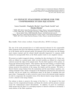
t
(xnw , ∆t)
(xne , ∆t)
Qne
Qnw
Qse
Qsw
(xsw , ∆t)
n
¯e
y
(xne , 0)
x
O
(xsw , 0)
(xse , 0)
Figure 7: Planes in the interior of the space-time volume Q.
Let us denote by n
¯ e = ne /kne k the unit normal of the plane Se that contains the three
points Qse , Qne , and O, as illustrated in Figure 7. Without diﬃculty, we identify the distinct
−−→
−−→
vectors OQne = (sne ∆t, sen ∆t, ∆t) and OQse = (sse ∆t, ses ∆t, ∆t) that lie on the ﬂat surface and
determine their cross product to compute the normal ne , namely
−−→
−−→
ne = OQne × OQse = ∆t2 [(sen − ses ) i − (sne − sse ) j + (sne ses − sen sse ) t] ,
(3.11)
with i, j and t the standard basis in the physical space (x, y, t). The Rankine-Hugoniot condition
across the discontinuity surface Se is then ne · (f ∗∗ − f ∗e , g ∗∗ − g ∗e , w∗∗ − w∗e ) = 0, obtained
by means of equation (3.4), which can be rewritten as
(sne ses − sen sse )(w∗e − w∗∗ ) + (sen − ses )(f ∗e − f ∗∗ ) + (sse − sne )(g ∗e − g ∗∗ ) = 0.
(3.12)
For the remaining directions, a similar procedure is employed to get the conditions across the
corresponding planes, and a summary of all, including (3.12), is presented below:
N
W
δw
δf
δg
δw
δf
δg
δw
δf
δg
δw
δf
δg
1
1
}|
{
{
z }|
z }|1 {
z
n e
w n
w
e
(sw sn − sn se )(wn∗ − w∗∗ ) + (sn − sn )(f n∗ − f ∗∗ ) + (sne − snw )(g n∗ − g ∗∗ )= 0, (3.13a)
2
2
z }|
z }|2 {
}|
{
{
z
s w
w n
w
w
(sw sn − ss sw )(w∗w − w∗∗ ) + (ss − sn )(f ∗w − f ∗∗ ) + (snw − ssw )(g ∗w − g ∗∗ )= 0, (3.13b)
3
3
z }|
z }|3 {
}|
{
{
z
s w
e s
e
w
S
(se ss − ss sw )(ws∗ − w∗∗ ) + (ss − ss )(f s∗ − f ∗∗ ) + (ssw − sse )(g s∗ − g ∗∗ )= 0, (3.13c)
E
4
4
z
z }|
z }|4 {
}|
{
{
n e
e s
e
e
(se ss − sn se )(w∗e − w∗∗ ) + (sn − ss )(f ∗e − f ∗∗ ) + (sse − sne )(g ∗e − g ∗∗ )= 0. (3.13d)
RR n° 8540
22
Vides, Nkonga & Audit
Relations (3.13) form a system of linear equations and, since the speciﬁc value of the strongly
interacting state w∗∗ is completely determined by equation (3.9), we opt to rewrite it as
δ1f f ∗∗ + δ1g g ∗∗ = δ1w (wn∗ − w∗∗ ) + δ1f f n∗ + δ1g g n∗ = b1 ,
f
g
f
w
g
(3.14a)
δ2 f ∗∗ + δ2 g ∗∗ = δ2 (w∗w − w∗∗ ) + δ2 f ∗w + δ2 g ∗w = b2 ,
δ3f f ∗∗ + δ3g g ∗∗ = δ3w (ws∗ − w∗∗ ) + δ3f f s∗ + δ3g g s∗ = b3 ,
(3.14b)
(3.14c)
δ4f f ∗∗ + δ4g g ∗∗ = δ4w (w∗e − w∗∗ ) + δ4f f ∗e + δ4g g ∗e = b4 ,
(3.14d)
with the unknown ﬂuxes on the left hand-side. It is evident that (3.14) is overdetermined, seeing
that there are four equations to solve for two unknowns, and the method of ordinary least squares
can be utilized to ﬁnd a solution. Hence, we express the linear system (3.14) in the form Ax = b,
by deﬁning


 w
 f
δ1 (wn∗ − w∗∗ ) + δ1f f n∗ + δ1g g n∗
δ1 δ1g
 δ2w (w∗w − w∗∗ ) + δ f f ∗w + δ g g ∗w 
δ f δ g 
f ∗∗
2
2
2
2


A=
δ3f δ3g  , x = g ∗∗ , and b = δ3w (ws∗ − w∗∗ ) + δ3f f s∗ + δ3g g s∗  , (3.15)
δ4w (w∗e − w∗∗ ) + δ4f f ∗e + δ4g g ∗e
δ4f δ4g
and write the normal equations in matrix notation as AT Ax = AT b. The least squares solution
x = M −1 AT b = Kb, provided M = AT A can be inverted, is the exact one if it exists or an
approximate one if it does not.
Considering that M has in fact a strictly positive determinant (A.3) and is consequently
nonsingular (see Annex A), we are thus able to get explicit forms for the ﬂuxes in the interaction
region as
f ∗∗ = [k11 b1 + k12 b2 + k13 b3 + k14 b4 ] / det M ,
(3.16)
g ∗∗ = [k21 b1 + k22 b2 + k23 b3 + k24 b4 ] / det M ,
(3.17)
given in terms of the matrix elements
k11 = δ1f (δ2g 2 + δ3g 2 + δ4g 2 ) − δ1g (δ2f δ2g + δ3f δ3g + δ4f δ4g ),
k12 = δ2f (δ1g 2 + δ3g 2 + δ4g 2 ) − δ2g (δ1f δ1g + δ3f δ3g + δ4f δ4g ),
k13 = δ3f (δ1g 2 + δ2g 2 + δ4g 2 ) − δ3g (δ1f δ1g + δ2f δ2g + δ4f δ4g ),
k14 = δ4f (δ1g 2 + δ2g 2 + δ3g 2 ) − δ4g (δ1f δ1g + δ2f δ2g + δ3f δ3g ),
2
2
2
2
2
2
2
2
2
2
2
2
k21 = δ1g (δ2f + δ3f + δ4f ) − δ1f (δ2f δ2g + δ3f δ3g + δ4f δ4g ),
k22 = δ2g (δ1f + δ3f + δ4f ) − δ2f (δ1f δ1g + δ3f δ3g + δ4f δ4g ),
k23 = δ3g (δ1f + δ2f + δ4f ) − δ3f (δ1f δ1g + δ2f δ2g + δ4f δ4g ),
k24 = δ4g (δ1f + δ2f + δ3f ) − δ4f (δ1f δ1g + δ2f δ2g + δ3f δ3g ).
(3.18)
The advantage of the suggested formulation over existing ones is that it eﬃciently encloses
all feasible subsonic or supersonic conﬁgurations for the two-dimensional interaction of waves
associated with the Riemann problem (2.25, 2.28), while providing a single and perspicuous
implementation of the approximated variables w∗∗ (3.9) and F ∗∗ (3.17).
If we regard the elements of the matrix K as weights, we notice that k11 , k13 , k22 and k24
become smaller as the strongly interaction region in the t = ∆t plane turns rectangular. In fact,
studying once more the situation discussed at the end of the previous section where this region is
a rectangle R′ , we perceive that in the limit sβα → sα for α, β ∈ {n, s, e, w}, δ1g = −δ3g , δ4f = −δ2f
Inria
A Simple 2D Extension of the HLL Riemann Solver for Gas Dynamics
23
and δ1f = δ3f = δ2g = δ4g = 0. This further implies that the four mentioned weights become zero
2
and k12 = 2δ2f δ1g 2 = −k14 , k21 = 2δ1g δ2f = −k23 , allowing us to ﬁnd
f ∗∗ =
g ∗∗ =
1
2
1
2
[(se + sw ) w∗∗ − se w∗e − sw w∗w + f ∗e + f ∗w ] ,
(3.19a)
[(sn + ss ) w∗∗ − sn wn∗ − ss ws∗ + g n∗ + g s∗ ] ,
(3.19b)
having substituted the quantities deﬁned in (3.13). Equations (3.19) aid to conﬁrm that our
proposed approach is able to pick out the right ingredients for the determination of the numerical
ﬂux F ∗∗ . It is worth observing that for this particular case, f ∗∗ (respectively, g ∗∗ ) is simply
the average of the jump conditions across the eastern and western (respectively, northern and
southern) planes of the inverted rectangular pyramid, as expected.
The above analysis inspired us to develop two alternative formulations to (3.17), which will
be duly justiﬁed in the subsequent section. For all details pertaining the appropriate use of the
resolved ﬂuxes at the primary cells’ interfaces, refer to Section 3.3.
3.2.3
Alternative Formulations
As the linear system (3.14) is mathematically overdetermined, we could theoretically propose
inﬁnitely many formulations to estimate F ∗∗ , not all of which would be sensible. However, in
this spirit, we detail two of which will give reasonable solutions and yield shorter expressions
than in (3.17), for later interpretation and implementation. The ﬁrst method gives ﬂuxes that
are dependent on the intermediate state w∗∗ , as opposed to the ones provided by the second.
Form I
We ﬁrst calculate the diﬀerence between equations (3.14a) and (3.14c), and separately, the one
between (3.14d) and (3.14b), to recover a system of two, not four, linear equations that can be
written in condensed form as
f
δ1 − δ3f δ1g − δ3g
f ∗∗
b1 − b3
,
(3.20)
=
δ4f − δ2f δ4g − δ2g
g ∗∗
b4 − b2
where the 2×2 real matrix on the left-hand side is denoted by AI . A straightforward substitution
of the terms introduced in (3.13) into this matrix allows us to compute its determinant as
det AI = − ∆t4 2 a∗∗ , which is certainly less than zero on the assumption that both ∆t and a∗∗ are
positive quantities. The unique solution of (3.20) is then
∆t2 sse + ssw − sne − snw snw + ssw − sne − sse
b1 − b3
f ∗∗
.
(3.21)
=−
e
w
w
e
e
b4 − b2
sw
g ∗∗
4a∗∗ ses + sw
s − sn − sn
n + ss − sn − ss
By substituting the constant one-dimensional states and ﬂuxes deﬁned in (2.34) and (2.35)
into the terms b1 − b3 and b4 − b2 , we obtain
n
w s
n e
s e
w n
n e
e s
s w
b1 − b3 = (sw
n se + ss se − sw sn − sw ss )w ∗∗ − sn se w ne + sw sn w nw + ss sw w sw − se ss w se
e
e
w
n
n
s
s
+ sw
n f ne − sn f nw − ss f sw + ss f se − (sw − se )g n∗ − (sw − se )g s∗ ,
n e
w n
s w
s e
w n
e n
s
b4 − b2 = (sen sse + sw
n sw − ss se − ss sw )w ∗∗ − se sn w ne − sw sn w nw + ss sw w sw + se ss w se
s
s
n
n
e
e
w
+ se g ne + sw g nw − sw g sw − se g se − (ss − sn )f ∗e − (ss − sw
n )f ∗w ,
so the ﬂuxes f ∗∗ and g ∗∗ possess a clear and condensed form. Note that in the limit sβα → sα ,
with α, β ∈ {n, s, e, w}, system (3.21) corresponds to (3.19).
RR n° 8540
24
Vides, Nkonga & Audit
Form II
We shall now describe a method that is built with the speciﬁc intention of eliminating the
contribution of the resolved state w∗∗ to the ﬂux tensor F ∗∗ . We start by summing equation
(3.13a) multiplied by δ3w and equation (3.13c) multiplied by −δ1w , to get
(δ1f δ3w − δ3f δ1w )f ∗∗ + (δ1g δ3w − δ3g δ1w )g ∗∗ = δ1w δ3w (wn∗ − ws∗ ) + δ1f δ3w f n∗
− δ3f δ1w f s∗ + δ1g δ3w g n∗ − δ3g δ1w g s∗ = c1 ,
(3.23)
and in an analogous manner, we multiply equation (3.13d) by δ2w and equation (3.13b) by −δ4w
so that their sum gives
(δ4f δ2w − δ2f δ4w )f ∗∗ + (δ4g δ2w − δ2g δ4w )g ∗∗ = δ4w δ2w (w∗e − w∗w ) + δ4f δ2w f ∗e
− δ2f δ4w f ∗w + δ4g δ2w g ∗e − δ2g δ4w g ∗w = c2 .
(3.24)
Using the same methodology as in Form I, we employ matrix notation to write both linear
equations as
f w
f ∗∗
δ1 δ3 − δ3f δ1w δ1g δ3w − δ3g δ1w
c1
,
(3.25)
=
g ∗∗
c2
δ4f δ2w − δ2f δ4w δ4g δ2w − δ2g δ4w
with the square matrix denoted by AII , which, if invertible, allows us to ﬁnd simple and compact
representations for the ﬂuxes f ∗∗ and g ∗∗ . We wish to point out that in actual practice, we have
not yet encountered a situation where AII is singular.
Additionally, it is interesting to observe the behavior of this method in the limit that has
hitherto been considered (sβα → sα for α, β ∈ {n, s, e, w}), where
sn g s∗ − ss g n∗ + sn ss (wn∗ − ws∗ )
,
sn − ss
(3.26)
which are clearly consistent and can be seen as one-dimensional HLL ﬂuxes (2.23) with initial
data that are HLL intermediate states themselves.
f ∗∗ =
3.2.4
se f ∗w − sw f ∗e + se sw (w∗e − w∗w )
se − sw
and g ∗∗ =
Consistency
In the next few paragraphs, we give various statements concerning the consistency of the proposed
numerical scheme, where w∗∗ is deﬁned by equation (3.9) and F ∗∗ by (3.17). For this, let us
¯ constant in x ∈ R2 , as well as w
¯ e, w
¯ n, w
¯ w , and w
¯ s constant in x > 0, y > 0,
deﬁne a state w
x < 0 and y < 0, respectively, with the corresponding ﬂuxes denoted in a similar way.
Given that the scheme is in conservative form, we need to verify if the numerical ﬂuxes are
¯ w,
¯ w,
¯ w)
¯ = f (w)
¯ and g ∗∗ (w,
¯ w,
¯ w,
¯ w)
¯ = g(w).
¯
consistent with the physical ones, i.e., if f ∗∗ (w,
Making use of equations (3.19) with the speeds deﬁned as se = sn = s = −ss = −sw , and
¯ w)
¯ = f (w),
¯
recalling the fact that the one-dimensional HLL ﬂuxes are consistent, e.g., f ∗e (w,
we surely recover that these basic consistency equalities are satisﬁed.
In addition, if all variations occur in one spatial direction, as depicted in Figure 8, equation
(3.9) reduces to an analogue of (2.16). For instance, if the variation is restricted to the y-direction,
¯ n = F ne = F nw and F
¯ s = F se = F sw ,
¯ n = wne = wnw , w
¯ s = wse = wsw , F
we are sure that w
and the equality (3.9) changes into
w∗∗ =
¯ n − ss w
¯ s − (¯
¯s)
sn w
gn − g
.
sn − ss
(3.27)
Inria
25
A Simple 2D Extension of the HLL Riemann Solver for Gas Dynamics
xnw
xne
xnw
xne
¯n
w
¯w
w
¯∗
w
sn ∆t
¯∗
w
¯e
w
ss ∆t
¯s
w
y xsw
sw ∆t
se ∆t
xse
x
y xsw
xse
x
(a) Variation in the x-direction
(b) Variation in the y-direction
Figure 8: Two-dimensional variations restricted to a single spatial direction.
3.3
Extensions and Computational Remarks
The goal of this section is to exhibit a general representation of the proposed solver for twodimensional meshes satisfying certain properties and simultaneously provide insight into its implementation. We then elaborate on how to assemble the total ﬂux across the mesh edges or
interfaces and on how to obtain a second-order version of the scheme.
3.3.1
Non-Rectangular Meshes
In the framework of ﬁnite volume methods, the technique presented in Section 3 naturally relies
on integral relations that can be easily applied over any right prism in the physical space (x, y, t).
So, let T be an admissible mesh deﬁned over an open bounded region Ω ∈ R2 in the sense of [12]
(Deﬁnition 9.1) consisting of polygonal cells Cc ∈ T (with c a unique index), edges, and vertices;
the latter belonging to a family denoted by P. Moreover, for each vertex p ∈ P, we construct a
dual convex cell Dp by connecting the centers of the polygons that share this point and establish
the space-time control volume Qp = Dp × (0, ∆t). An integration of (2.25) over this prism Qp
then yields the expression
Z
Z
Z
∇ · F (w(x, t)) dx dt = 0,
(3.28)
w(x, 0) dx +
w(x, ∆t) dx −
Qp
Dp
Dp
with F = (f , g) and x = (x, y), which is known to be equivalent to
Z
Z
Z
w(x, ∆t) dx =
w(x, 0) dx −
F (w(s, t)) · dS,
Dp
Dp
(3.29)
Sp
by application of the divergence theorem, given Sp = ∂Dp × (0, ∆t). For presentation purposes,
we shall hereafter limit ourselves to the case where Dp is a basic triangle. However, we urge
the reader to keep in mind that all subsequent developments can be readily generalized to any
convex polygonal dual cell.
Thus, we consider the volume Qp to be a triangular prism, provided Dp is adequately deﬁned
by joining together the three distinct centers
xα = (xα , yα ),
RR n° 8540
α = 1, 2, 3,
(3.30)
26
Vides, Nkonga & Audit
t
1∆
sr
1
sl
r
L1
∆t
l
L1
w ∗1
C1
C2
x2
Dp
x1
L1
ν1
w1
s3l ∆t
w∗∗
p
w2
w ∗3
s3r ∆t
w3
C3
y
y
w ∗2
sr2
∆t
x3
s2
l ∆
t
x
x
(a) Global view of possible structures
(b) Zoom on a triangular dual cell
Figure 9: A solution example at time t = ∆t, resulting from the application of HLL Riemann
solvers at the interfaces and at the vertices of the underlying non-rectangular mesh.
of the corresponding primary cells Cα , as exempliﬁed in Figure 9. Owing to its construction,
the dual cell contains the vertex p that is evidently the intersection point of three edges Lα , for
which we know their respective formulations and unit normals ν α = (ναx , ναy ). We employ the
notation Lα to designate the line segment having p as one of its endpoints and lying between xα
and xα+1 , with the index α following a cyclic order such that for α = 3, α + 1 = 1.
As explained in Section 2.2, a constant state wα is assumed within each cell Cα at the initial
time t0 ≥ 0, for α = 1, 2, 3. Using now Figure 9(b) as reference, it is evident that in order to
obtain the desired values at the face Lα × (t0 , t0 + ∆t) in the interior of Qp , we must solve not
only a one-dimensional Riemann problem in its normal direction, but also a local two-dimensional
Riemann problem, involving initial data w1 , w2 and w3 , at the vertex p.
α
For the former, we identify as sα
l and sr the left and right HLL wave speeds in the direction
of ν α , after making use of equation (2.24) with wl = wα+1 and wr = wα . Moreover, solving the
one-dimensional Riemann problems at the edges allows us to derive expressions for the constant
state w∗α (2.16) and HLL ﬂuxes (2.23) associated with each problem, i.e.,
α
sα
r w α − sl w α+1 + ν α · (F α+1 − F α )
,
α
sα
r − sl
α
α α
ν α · (sα
r F α+1 − sl F α ) + sl sr (w α − w α+1 )
=
,
α
α
sr − sl
w∗α =
(3.31a)
f n∗α
(3.31b)
where f n∗α = ν α · F ∗α is the ﬂux perpendicular to the edge α ∈ {1, 2, 3}. We recall that the
transverse ﬂuxes, denoted here as f n∗α⊥ = (−ναy , ναx )·(f ∗α , g ∗α ), can be constructed using values
extracted from the associated normal ﬂux (3.31b) and intermediate state (3.31a), as was done in
Section 2.2.2. In addition, we easily recover the two parallel lines that bound the extent of w∗α
on the xy-plane at some time t > t0 , which are given by
Lrα (t) = {(x, y) | ναx x + ναy y = sα
r (t − t0 )} ,
(3.32a)
Llα (t)
(3.32b)
= {(x, y) | ναx x + ναy y =
sα
l
(t − t0 )} ,
Inria
27
A Simple 2D Extension of the HLL Riemann Solver for Gas Dynamics
having conveniently set p = (0, 0) and recalling that kν α k = 1. From now on, we also consider
the time t = ∆t and t0 = 0.
With regard to the two-dimensional Riemann problem found at the origin O = (p, 0), we
specify a triangular region by connecting the vertices q α = (x′α ∆t, yα′ ∆t), for α = 1, 2, 3, which
are essentially the intersection points of the bounding lines Llα (∆t) and Lrα+1 (∆t) such that
x′α =
ναy − sα
sα+1
r
l ν(α+1)y
ν(α+1)x ναy − ναx ν(α+1)y
and yα′ =
α+1
sα
ναx
l ν(α+1)x − sr
.
ν(α+1)x ναy − ναx ν(α+1)y
(3.33)
Let us note that all two-dimensional complex interactions emanating from O and projected onto
the planar surface t = ∆t, are well-contained in the previously mentioned triangle, which in turn
generates an inverted triangular pyramid during its time evolution from 0 to ∆t.
The previous statements facilitate the derivation of an algebraic equation to compute the
constant state w∗∗ , when applying the integral conservation law (3.29) over the control volume
Qp . However, for the determination of the ﬂux f ∗∗ , we still need to provide the Rankine-Hugoniot
relations that hold across the surfaces of discontinuities emerging from O, following the approach
carefully detailed in Section 3.2.2. We therefore start by identifying the points Qα = (q α , ∆t)
and the normals
′
−−→
−−→
′
) t , (3.34)
nα = OQα+1 × OQα = ∆t2 (yα+1
− yα′ ) i + (x′α − x′α+1 ) j + (x′α+1 yα′ − x′α yα+1
that will allow us to deduce the jump conditions for α = 1, 2, 3 as
δw
δf
δg
α
α
α
z
z
z
}|
{
}|
{
}|
{
′
′
′
′
′ ′
′
(xα+1 yα − xα yα+1 )(w∗α − w∗∗ ) + (yα+1 − yα )(f ∗α − f ∗∗ ) + (xα − x′α+1 )(g ∗α − g ∗∗ ) = 0, (3.35)
which can be written in the following form:
δαf f ∗∗ + δαg g ∗∗ = δαw (w∗α − w∗∗ ) + δαf f ∗α + δαg g ∗α = bα ,
α = 1, 2, 3.
(3.36)
Clearly, relations (3.36) form once again an overdetermined system of linear equations, since
there are more equations (three) than unknowns (two). In view of the method of ordinary least
squares, we then express this system as AT x = bT by deﬁning
 f

 w

δ1 δ1g
δ1 (w∗1 − w∗∗ ) + δ1f f ∗1 + δ1g g ∗1
f ∗∗
AT = δ2f δ2g  , x =
, and bT = δ2w (w∗2 − w∗∗ ) + δ2f f ∗2 + δ2g g ∗2  , (3.37)
g ∗∗
f
g
δ3 δ3
δ3w (w∗3 − w∗∗ ) + δ3f f ∗3 + δ3g g ∗3
and look for the least squares solution x = M T −1 AT T bT , provided M T is invertible. It is worth
mentioning that in the general case when three or more edges (ε ≥ 3) meet at the vertex p, the
matrix


X
X 2

δαf δαg 
δαf




α=1,...,ε
(3.38)
M T =  α=1,...,ε
,
X

 X
g2
f g


δ
δ δ
α α
α=1,...,ε
α
α=1,...,ε
has a determinant that can be expressed as the sum of square binomials of the form (δαf δβg −δβf δαg )2 ,
for all α, β ∈ {1, 2, . . . , ε}, which is geometrically proven to be strictly positive as long as the
area of the interaction region a∗∗ is not zero.
Hence, we conﬁrm that the proposed approach is simple enough to be applied on any admissible mesh, yielding useful closed expressions for the intermediate state w∗∗ and ﬂux F ∗∗ .
RR n° 8540
28
3.3.2
Vides, Nkonga & Audit
Flux Assembling at Faces
The assembling of the total ﬂux at the cells’ faces is an important aspect that has to be carefully
considered. Although we perform the subsequent study focusing on the rectangular mesh used in
Section 3, we note that all formalisms developed here can be easily adapted to other conﬁgurations
such as the ones presented in the previous section.
After analyzing the structures shown in Figures 2(a) and 9(a), we can infer that the ﬁnal
expression will be a convex combination of one-and two-dimensional ﬂuxes, as in [3, 5, 19]. Each
ﬂux at an edge of the primary cell Ci,j can be obtained from the surface average of the ﬂux
normal to the underlying space-time face, e.g.,
Z y 1 Z ∆t
j+
1
2
φx,i+ 12 ,j =
F (w(xi+ 21 , t)) · n
¯ i+ 12 dt dy,
(3.39)
∆y ∆t yj− 1 0
2
being n
¯ i+ 12 = (1, 0) the unit normal vector of Si+ 12 = (yj− 21 , yj+ 21 ) × (0, ∆t).
In the subsonic case, the above deﬁnite integral can be evaluated by considering the contributions at the face coming from the one- and two-dimensional Riemann solvers initially applied
at the cell’s edge and vertices, respectively. The averaged ﬂux becomes
hll2D
hll
hll2D
φx,i+ 21 ,j = θs,i+ 12 ,j+ 21 φx,i+
1
,j+ 1 + θy,i+ 12 ,j φx,i+ 1 ,j + θn,i+ 21 ,j− 21 φx,i+ 1 ,j− 1 ,
2
2
2
2
2
(3.40)
with
θs,i+ 12 ,j+ 21 =
∆t
ss,i+ 21 ,j+ 12 |,
2 ∆y |ˆ
and
θn,i+ 12 ,j− 21 =
∆t
sn,i+ 21 ,j− 12 |,
2 ∆y |ˆ
θy,i+ 21 ,j = 1 − θs,i+ 12 ,j+ 12 − θn,i+ 21 ,j− 12 .
It is obvious that the weights θs,i+ 12 ,j+ 21 and θn,i+ 12 ,j− 21 determine the amount of two-dimensional
contributions that the total ﬂux at the cell’s face will possess, and they are directly linked through
the time step with the CFL number used in practice (for details regarding the associated CFL
condition, we refer the reader to [3, p. 1977] where it is fully explained). We remark that a
simpler alternative to (3.40) is ﬁxing the weights to the coeﬃcients in Simpson’s rule, used to
numerically integrate the average of F (w(xi+ 12 , ∆t)) · n
¯ i+ 12 over the edge (yj− 21 , yj+ 21 ), yielding
φx,i+ 21 ,j =
1
6
hll2D
φx,i+
1
,j+ 1 +
2
2
4
6
φhll
x,i+ 1 ,j +
2
1
6
hll2D
φx,i+
1
,j− 1 .
2
2
(3.41)
Let us note that in equations (3.40) and (3.41), we have employed new variables that need
to be appropriately deﬁned. First, the element having the superscript “hll” is essentially the
one-dimensional numerical ﬂux described in equation (2.21), but with a two-dimensional index
hll
n
n
instead, such that φhll
x,i+ 1 ,j = φ (wi,j , wi+1,j ). In a similar manner, we specify
2
hll2D
hll2D
(wni+1,j+1 , wni,j+1 , wni,j , wni+1,j ),
φx,i+
1
,j+ 1 = φx
2
2
hll2D
φx,i+
1
1
2 ,j− 2
=
φxhll2D (wni+1,j
,
wni,j
,
wni,j−1
,
wni+1,j−1 ),
(3.42a)
(3.42b)
hll2D
where φx,m,n
is the local ﬂux f ∗∗ of the two-dimensional Riemann problem deﬁned at the vertex
xm,n , with analogous considerations for the y direction. Next, the wave speeds denoted by sˆα ,
for α ∈ {n, s, e, w}, are determined from the intersection of the interaction region with the xand y-axes at time ∆t (notice the circles pictured in Figure 3(b) of Section 2.2.1), speciﬁcally
e
w
ss − sw
sn − sen
s
e
s
w
n
,
sˆs = ss − se
,
sˆn = sn − sw
sn − sne
sse − ssw
nw
(3.43)
sw − ssw
sse − sne
s
w
n
e
sˆw = sw − ss
,
sˆe = se − sn
,
w
sw
ses − sen
n − ss
Inria
29
A Simple 2D Extension of the HLL Riemann Solver for Gas Dynamics
and in the limit sβα → sα for α, β ∈ {n, s, e, w}, sˆα = sα .
Equations (3.40) and (3.41) are strictly valid only for a ﬂow that is subsonic everywhere.
+
s−
w−
However, if we reformulate our signal speeds deﬁned in (2.32) as sne + , sen+ , snw− , sw
n , sw , ss
s+
e−
se , and ss , and utilize them to recover all one- and two-dimensional states and ﬂuxes associated
with our multidimensional Riemann solver (2.34, 2.35, 2.48, 3.9, 3.17), we are able to account
for supersonic situations and employ both (3.40) and (3.41) without any additional adjustments.
hll2D
Another way to deal with supersonic situations is to approximately deﬁne the ﬂuxes φx,m,n
hll2D
and φy,m,n as the upwinded ﬂuxes at the space-time point (xm,n , ∆t), as given in [4, p. 7483]
and partially described in equation (2.54). Henceforth, we use the term Simpson assembling to
denominate equation (3.41) together with these upwinded 2D ﬂuxes.
The most accurate approach to handle supersonic ﬂows is to manually track the position of
the interaction region and deduce the actual elements that contribute to the total ﬂux at each
of the cell’s faces. For instance, on examining the conﬁguration shown in Figure 6(a), it is clear
that for this example, f ∗∗ does not have an eﬀect in the total ﬂux assembled at the vertical edge,
and choosing f ∗w when assembling would certainly be more accurate. For this, we choose to
introduce a new expression
hll
e
e hll2D1 1 + θe
e hll2D
φx,i+ 21 ,j = θes,i+ 21 ,j+ 12 φ
y,i+ 21 ,j φx,i+ 1 ,j + θn,i+ 12 ,j− 12 φx,i+ 21 ,j− 21 ,
x,i+ 2 ,j+ 2
2
where
θes,i+ 12 ,j+ 21 =
∆t
ss,i+ 21 ,j+ 12 |,
2 ∆y |˜
and
θen,i+ 21 ,j− 12 =
(3.44)
∆t
sn,i+ 12 ,j− 21 |,
2 ∆y |˜
θey,i+ 12 ,j = 1 − θes,i+ 21 ,j+ 12 − θen,i+ 21 ,j− 21 .
e hll2D needs to be regarded as a convex combination of local ﬂuxes asHere, the x-directional ﬂux φ
x,m,n
sociated to the nine states, characterized by the set Lm,n = {∗∗, n∗, s∗, ∗e, ∗w, ne, nw, sw, se},
of the two-dimensional Riemann solver centered at xm,n , i.e.,
n
n
n
e hll2D (wn
e hll2D1 1 = φ
φ
x
i+1,j+1 , wi,j+1 , wi,j , wi+1,j ) =
x,i+ 2 ,j+ 2
X
βy,µν f µν ,
(3.45a)
(µν) ∈ Li+ 1 ,j+ 1
e hll2D1 1
φ
x,i+ 2 ,j− 2
=
P
e hll2D (wn
φ
x
i+1,j
, wni,j , wni,j−1 , wni+1,j−1 ) =
X
2
2
βy,µν f µν ,
(3.45b)
(µν) ∈ Li+ 1 ,j− 1
2
2
and βy,µν ≥ 0,
βy,µν = 1, with similar equations and notation for the y-direction. Each
coeﬃcient βy,µν corresponds to the fraction of the interaction surface associated to the local
state µν. In a subsonic conﬁguration, notice that only βy,∗∗ = 1 and all others are zero.
Equation (3.44) will now be referred to as manual assembling and in Annex B, we provide
the speciﬁc details for the implementation of (3.44, 3.45) with the help of pseudocode. There, we
observe that the third algorithm corresponds to the approximate (due to some simpliﬁcations)
two-dimensional analogue of having written equation (2.20) as

if 0 < sl ,

 fl
if sl < 0 < sr ,
(3.46)
φhll (wl , wr ) = f ∗


fr
if 0 > sr .
3.3.3
Predictor-Corrector Scheme of Second-Order Accuracy
The ﬁrst order scheme is now complete and the next step is to deﬁne an appropriate second-order
extension. This is achieved by means of a simple predictor-corrector approach similar to the one
RR n° 8540
30
Vides, Nkonga & Audit
proposed by Balsara in [3, 4], which roughly consists of using the two-dimensional Riemann
solver for both steps involved in the algorithm. A consequence of employing this solver in the
corrector step is the introduction of more isotropy into the simulation. Instead, “our use of the
multidimensional Riemann solver in the predictor step has the happy consequence of raising the
maximal CFL number”, in the words of the author of [4], and we add the phrase “when needed”.
In the predictor step, the vector w is spatially reconstructed from the center of the primary
cell to its corners or vertices following a MUSCL-type approach, i.e., using piecewise linear
interpolations with slope limiters such as the MC limiter [35], minmod [31] or the positive
preserving limiter [34]. The reconstruction provides the four states that are necessary to solve
the multidimensional Riemann solver (2.34, 2.35, 2.48, 3.9, 3.17) at each corner, yielding the xand y-directional ﬂuxes that will contribute to the assembling at the cell’s faces. Now, to avoid
the appearance of spurious solutions for certain second-order simulations, we propose employing
e hll2D 1 1 + θe
e hll
e hll2D
e
φx,i+ 12 ,j = θey,i+ 12 ,j+ 12 φ
y,i+ 21 ,j φx,i+ 21 ,j + θy,i+ 12 ,j− 12 φxn ,i+ 12 ,j− 21 ,
xs ,i+ 2 ,j+ 2
(3.47)
where
θey,i+ 12 ,j± 21 =
ζ∆t
2 ∆y
sn,i+ 12 ,j± 21 |)
max(|˜
ss,i+ 21 ,j± 12 |, |˜
and
θey,i+ 12 ,j = 1 − θey,i+ 12 ,j+ 12 − θey,i+ 21 ,j− 12 ,
with analogous expressions for the other main direction. We note that we have introduced new
variables “hll2D” which are deﬁned in a way similar to (3.45) but with a diﬀerent subscript
that denotes the location relative to the local vertices (we refer the reader to Algorithm 4 in
e hll 1 at the
Annex B for more details regarding their precise deﬁnition). Moreover, the ﬂux φ
x,i+ 2 ,j
center of the face is simply the average of the nearest two x-directional HLL ﬂuxes, one initially
computed below the vertex xi+ 21 ,j+ 12 and the other above xi+ 21 ,j− 12 , as partial inputs for our
two-dimensional Riemann solver. We then utilize the total assembled ﬂuxes to estimate the
vector of conservative variables at the half time step tn + ζ ∆t, with ζ = 21 .
For the corrector step, we repeat the operations carried out in the predictor step but having
set ζ = 1. The slopes computed at time tn are now applied to spatially reconstruct variables
that are centered both in time and space, i.e., the output of the predictor step.
In the coming section, we will present several numerical tests that were obtained with this
simple yet second-order accurate predictor-corrector approach. First-order approximations can
be obtained using the same computer code, by performing only one step with unreconstructed
states and ζ = 1.
4
Numerical Results
The purpose of this section is to validate our scheme with several multidimensional test problems
on a uniform rectangular mesh. The numerical implementation of our solver and Balsara’s [4]
(hereafter referred to as BAL2012) has been done in the HERACLES code [26] for astrophysical
ﬂuid ﬂows. By having a common computational framework, we can fairly compare the accuracy
and robustness of both methods.
We note that employing Simpson assembling at the cells’ faces for our solver yields almost the
exact same results as BAL2012, for which this type of assembling is the default for second-order
approximations, and thus, unless stated otherwise, we opt to display our method’s solutions with
the manual assembling (3.47). All tests were run with a CFL number of 0.9 and making use of
the predictor-corrector scheme mentioned in Section 3.3.3. As for the choice of slope limiters, we
applied the MC limiter [35] for all except the last (Section 4.4), where minmod [31] was utilized
instead.
Inria
31
A Simple 2D Extension of the HLL Riemann Solver for Gas Dynamics
4.1
Accuracy Analysis
We wish to estimate the rate at which the L1 error for the proposed scheme decreases as the
numerical grid is reﬁned. For this, we consider the initial density proﬁle [18]
ρ0 (x, y) = 1 + 0.2 sin(π(x + y)),
(4.1)
together with the velocities and pressure deﬁned in Section 4.1 of [24], i.e., u0 = 1, v0 = −0.5
and p0 = 1. The simulation is run to time t = 4, which corresponds to the time it takes for the
wave to be advected once around the periodic domain spanning [0, 2] × [0, 2]. The ﬁnal state is
then compared with the analytical one.
Scheme with Manual Asmb.
L1 error
L1 error
4.1098e-01
0.25
4.2679e-01
0.21
2.8650e-01
0.52
3.0515e-01
0.48
Resolution
None
25 × 25
4.8975e-01
50 × 50
100 × 100
MM [31]
PP [34]
MC [35]
Scheme with Simpson Asmb.
L1 order
Limiter
L1 order
4.9536e-01
200 × 200
1.7279e-01
0.73
1.8704e-01
0.71
400 × 400
9.5487e-02
0.86
1.0429e-01
0.84
800 × 800
5.0278e-02
0.93
5.5167e-02
0.92
1600 × 1600
2.5808e-02
0.96
2.8383e-02
0.96
25 × 25
2.0198e-01
50 × 50
6.5074e-02
1.63
6.7657e-02
2.1682e-01
1.68
100 × 100
2.8358e-02
1.20
3.0418e-02
1.15
200 × 200
7.8803e-03
1.85
8.4898e-03
1.84
400 × 400
2.1739e-03
1.86
2.3589e-03
1.85
800 × 800
5.9648e-04
1.87
6.4860e-04
1.86
1600 × 1600
1.5876e-04
1.91
1.7275e-04
1.91
25 × 25
7.7416e-02
7.9507e-02
50 × 50
2.5379e-02
1.61
2.3234e-02
1.77
100 × 100
5.5017e-03
2.21
5.1137e-03
2.18
200 × 200
1.1486e-03
2.26
1.0969e-03
2.22
400 × 400
2.3008e-04
2.32
2.2597e-04
2.28
800 × 800
4.5417e-05
2.34
4.5906e-05
2.30
1600 × 1600
8.9790e-06
2.34
9.4001e-06
2.29
25 × 25
3.2846e-02
4.2989e-02
50 × 50
4.4552e-03
2.88
5.8172e-03
2.89
100 × 100
8.8114e-04
2.34
1.0172e-03
2.52
200 × 200
2.0742e-04
2.09
2.1494e-04
2.24
400 × 400
4.8755e-05
2.09
4.8707e-05
2.14
800 × 800
1.1452e-05
2.09
1.1523e-05
2.08
1600 × 1600
2.7050e-06
2.08
2.7568e-06
2.06
Table 1: L1 density errors and orders of accuracy for the wave advection test, using our proposed
scheme with diﬀerent slope limiters.
In Table 1, the accuracy results for our scheme are summarized. For both assembling methods
being compared, the L1 density errors decrease as the numerical resolution increases and we are
able to see that the lowest values are obtained when the MC limiter and manual assembling are
RR n° 8540
32
Vides, Nkonga & Audit
present. In addition, we observe that second-order accuracy is reached when any of the three
selected limiters are used, as was previously mentioned in Section 3.3.3. We mention that our
method with Simpson assembling not only gives roughly the same results as BAL2012 (e.g.,
diﬀerences after the seventh or eight decimal place for the MC limiter results) but also takes the
same amount of CPU time to complete with HERACLES.
1D HLL Solvers Only
L1 error
25 × 25
50 × 50
100 × 100
200 × 200
400 × 400
800 × 800
1600 × 1600
4.2162e-02
6.5289e-03
1.3566e-03
3.5122e-04
8.7975e-05
2.1608e-05
5.2697e-06
2.69
2.27
1.95
2.00
2.03
2.04
L1 order
Table 2: Density errors measured in the L1 norm for the wave advection test using the MC
limiter and one-dimensional HLL Riemann solvers in both the predictor and corrector steps.
The advantage, in terms of accuracy, of taking into account the multidimensional contributions for this problem is evident when we compare the rows corresponding to the MC limiter in
Table 1 with those of Table 2. The latter were obtained utilizing only 1D HLL Riemann solvers
in both steps of the predictor-corrector algorithm.
4.2
Multidimensional Riemann Problems
Density at t =0.52
Density at t =0.52
1.62
1.62
1.50
0.5
1.50
0.5
1.38
1.38
1.14
0.0
1.26
y
y
1.26
1.14
0.0
1.02
0.90
−0.5
0.78
1.02
0.90
−0.5
0.78
0.66
−0.5
0.0
x
0.5
0.54
0.66
−0.5
0.0
x
0.5
0.54
Figure 10: Density variable ρ obtained using BAL2012 (left, ρ:0.53-1.72) and our scheme (right,
ρ:0.53-1.71) for the MultiD RP1; computations performed on a 400 × 400 grid and 30 contour
lines displayed from 0.54 to 1.70 with a step of 0.04.
Firstly, we consider the two-dimensional problem described in [5, p. 183], with initial data given
in Table 3 (left). This Riemann problem (RP) initially consists of two contact discontinuities J
−
→
−
→
−
→
and two forward shock waves S , speciﬁcally S 21 J32 J34 S 41 borrowing the notation used in [32].
In general, we expect that both slip lines encounter the sonic circle of the constant state in the
third quadrant of the xy-plane and bend to end in spirals inside the subsonic area of the circle’s
−
→
−
→
portion lying in this quadrant. In addition, from the interaction of the shocks S 21 and S 41 , we
await the appearance of a pair of three-shock conﬁgurations, such that part of the subsonic area
is bounded by two joining Mach shocks and two reﬂected shocks.
Inria
33
A Simple 2D Extension of the HLL Riemann Solver for Gas Dynamics
Multidimensional Riemann Problems 1 & 2
Quadrant
ρ0 (x, y)
u0 (x, y)
v0 (x, y)
p0 (x, y)
ρ0 (x, y)
v0 (x, y)
p0 (x, y)
x > 0, y > 0
0.5313
0.0
0.0
0.4
1.0
u0 (x, y)
0.75
−0.5
1.0
x < 0, y > 0
1.0
0.7276
0.0
1.0
2.0
0.75
0.5
1.0
x < 0, y < 0
0.8
0.0
0.0
1.0
1.0
−0.75
0.5
1.0
x > 0, y < 0
1.0
0.0
0.7276
1.0
3.0
−0.75
−0.5
1.0
Computational domain: [−1, 1] × [−1, 1]; Free-flow boundary conditions
Table 3: Initial data for the ﬁrst MultiD RP described in [5] and the sixth of [20].
Multidimensional Riemann Problem 3
Quadrant
ρ0 (x, y)
u0 (x, y)
v0 (x, y)
p0 (x, y)
x > 0, y > 0
1.5
0.0
0.0
1.5
x < 0, y > 0
0.5323
1.206
0.0
0.3
x < 0, y < 0
0.1379
1.206
1.206
0.029
x > 0, y < 0
0.5323
0.0
1.206
0.3
Computational domain: [−1, 1] × [−1, 1]; Free-flow boundary conditions
Table 4: Initial data for the second MultiD RP described in [4].
By means of the contour plots shown in Figures 10 and 11, we can analyze the solutions of this
MultiD Riemann problem, computed on uniform grids of 4002 and 10002 cells, for both methods
being compared. All results follow the expected behavior described in the above paragraph, with
the additional property of being symmetric with respect to the x = y line, as was also anticipated.
There is no signiﬁcant diﬀerence between the plots obtained with the manual assembling and
those of BAL2012 for this particular test. Let us note that the low resolution of the contact
discontinuities is not surprising given that both methods are based on the two-wave model of the
HLL Riemann solver.
Density at t =0.52
Density at t =0.52
1.62
1.62
1.50
0.5
1.50
0.5
1.38
1.38
1.14
0.0
1.26
y
y
1.26
1.14
0.0
1.02
1.02
0.90
0.5
0.90
0.5
0.78
0.78
0.66
0.66
0.54
0.5
0.0
x
0.5
0.54
0.5
0.0
0.5
x
Figure 11: The density computed with BAL2012 (left) and our scheme (right) for MultiD RP1,
using 1000 × 1000 cells on 64 processors; contour lines chosen as in Fig. 10 (ρ:0.53-1.73).
−−−−−−−−−→
Next, we study the multidimensional Riemann problem J21 J32 J34 J41 that involves only slip
line initial data, summarized on the right of Table 3. Particularly, we expect the solutions to have
a vortex-type structure that turns in clockwise direction, with contact discontinuities spiraling
RR n° 8540
34
Vides, Nkonga & Audit
around the center, and this is the case for the numerical results presented in Figure 12. We can
observe that the ripples that are created in the ﬁrst and third quadrants of the left plot have
comparable resolution to those found in [20, 21, 32]. The detail of the ripples and slip lines is
greatly improved when the number of zones is increased, e.g., to one million cells, as shown in
the right image. We wish to mention that once again there is no visible diﬀerence between the
contours obtained with our scheme and the ones acquired with BAL2012, and this is the reason
why we only displayed the former.
Density at t =0.60
0.5
Density at t =0.60
2.95
2.95
2.65
2.65
2.35
0.5
2.35
1.75
0.0
2.05
1.75
y
y
2.05
0.0
1.45
1.45
1.15
−0.5
1.15
0.5
0.85
0.85
0.55
−0.5
0.0
x
0.5
0.55
0.25
0.25
0.5
0.0
0.5
x
Figure 12: Density ρ obtained using our scheme for MultiD RP2 on 400 × 400 (left, ρ:0.23-3.07)
and 1000 × 1000 (right, ρ:0.16-3.06) grids; 29 contour lines displayed from 0.25 to 3.05 with a
step of 0.10.
Density at t =1.10
Density at t =1.10
1.56
1.56
1.36
0.5
1.36
0.5
0.96
0.0
1.16
y
y
1.16
0.96
0.0
0.76
0.56
−0.5
0.76
0.56
−0.5
0.36
−0.5
0.0
x
0.5
0.16
0.36
−0.5
0.0
x
0.5
0.16
Figure 13: Contour plots of the density ρ obtained employing BAL2012 (left) and our scheme
(right) for the MultiD RP3; computations done on a 400×400 grid and 32 contour lines displayed
from 0.16 to 1.71 with a step of 0.05 (ρ:0.14-1.76).
Our last multidimensional Riemann problem, initially consisting of four backward shock waves
←
− ←
− ←
− ←
−
S 21 S 32 S 34 S 41 , is the most severe of the tests presented in this subsection. Its initial and
boundary conditions are given in Table 4. The expected behavior of this problem is properly
speciﬁed in Conﬁguration 3 of [32]. Here, we brieﬂy mention that during its time evolution, the
solution develops a double Mach reﬂection and a shock propagates in the southwest direction
Inria
35
A Simple 2D Extension of the HLL Riemann Solver for Gas Dynamics
at a 45-degree angle to the grid lines. This can be appreciated in Figures 13 and 14, where we
display the density variable ρ at time t = 1.1 by means of contour plots obtained with our scheme
and BAL2012, on two diﬀerent meshes. Clearly, the region of strong and complex interactions
associated with the problem is located in the third quadrant, where we are able to observe a
well-resolved mushroom cap (especially in the ﬁner grid where it is sharp), which is consistent
with expectations. Once more, all solutions are visually symmetric with respect to x = y.
Density at t =1.10
Density at t =1.10
1.56
1.56
1.36
0.5
1.36
0.5
0.96
0.0
1.16
y
y
1.16
0.96
0.0
0.76
0.76
0.56
0.5
0.56
0.5
0.36
0.36
0.16
0.5
0.0
0.16
0.5
0.5
x
0.0
0.5
x
Figure 14: Density estimated with BAL2012 (left) and our scheme (right) for MultiD RP3, using
1000 × 1000 cells on 64 proc.; contours chosen as in Fig. 13 (ρ:0.14-1.75).
We wish to note that if we do not properly assemble the ﬂux at each cell’s faces for this
problem, second-order computations will suﬀer from the spurious solution known as the carbuncle
phenomenon. In fact, prevention of this instability is what inspired us to derive and recommend
equation (3.47) instead of (3.40) for the assembling (Algorithms 3 and 2 in Annex B, respectively).
For ﬁrst-order approximations, both mentioned expressions are equivalent; the results shown in
Figure 15 were created using extremely ﬁne meshes of 16 million and 100 million cells, proving
the robustness of the ﬁrst-order scheme.
Density at t =1.10
Density at t =1.10
1.56
1.56
1.36
0.5
1.36
0.5
0.96
0.0
1.16
y
y
1.16
0.96
0.0
0.76
0.56
0.5
0.76
0.56
0.5
0.36
0.36
0.16
0.5
0.0
x
0.5
0.16
0.5
0.0
0.5
x
Figure 15: First-order density results for MultiD RP3 obtained with our scheme on 4000 × 4000
(left, 512 processors) and 10000 × 10000 (right, 1024 processors) cells; contours chosen as in Fig.
13 (ρ:0.14-1.75).
RR n° 8540
36
Vides, Nkonga & Audit
4.3
Double Mach Reflection
The double Mach reﬂection problem proposed by Woodward and Colella [38] starts oﬀ as a Mach
10 oblique shock in air encountering a reﬂecting wall. Using the set-up originally given in [38], we
run the simulation until the ﬁnal time t = 0.2 for the range of resolutions considered by Balsara
[3, 4], i.e., grids consisting of 960 × 240, 1920 × 480 and 2400 × 600 zones, spanning the domain
[0, 4] × [0, 1].
Density at t =0.20
Density at t =0.20
0.8
22.44
22.44
19.86
19.86
0.8
y
y
0.6
0.4
0.2
17.27
17.27
14.69
0.6
14.69
12.11
12.11
0.4
9.52
9.52
6.94
6.94
0.2
4.35
4.35
1.77
0.0
0.5
1.0
1.5
2.0
2.5
3.0
0.0
1.77
0.5
1.0
x
1.5
2.0
2.5
3.0
x
Density at t =0.20
Density at t =0.20
0.8
22.44
22.44
19.86
19.86
0.8
y
y
0.6
0.4
0.2
17.27
17.27
14.69
0.6
14.69
12.11
12.11
0.4
9.52
9.52
6.94
6.94
0.2
4.35
4.35
1.77
0.0
0.5
1.0
1.5
2.0
2.5
3.0
0.0
1.77
0.5
1.0
x
1.5
2.0
2.5
3.0
x
Density at t =0.20
Density at t =0.20
0.8
22.44
22.44
19.86
19.86
0.8
y
y
0.6
0.4
0.2
17.27
17.27
14.69
0.6
14.69
12.11
12.11
0.4
9.52
9.52
6.94
6.94
0.2
4.35
4.35
1.77
0.0
0.5
1.0
1.5
x
2.0
2.5
3.0
0.0
1.77
0.5
1.0
1.5
2.0
2.5
3.0
x
Figure 16: Results for the double Mach reﬂection problem obtained with BAL2012 (left) and
our scheme (right), using 25 density contours ranging from 1.77 to 22.44 with a constant step;
computations performed on 960×240 (top), 1920×480 (middle) and 2400×600 (bottom) meshes,
64 processors. All results have been plotted up to x = 3.
Figure 16 shows twenty-ﬁve density contours obtained with the two methods being compared,
on the above-mentioned meshes. We are able to see that the jet formed by the double Mach
reﬂection is well captured, especially on the ﬁnest grid; in all plots, we can observe the slipping
contact line that leads around to the forward moving Mach stem, which rolls-up creating a vortex
head. For the single-step Eulerian MUSCL results found in Figure 9e of [38], Woodward and
Colella provided an explanation for the oscillations and noise present near the slowly moving
shock, which we now quote as it directly applies to our case: “the shocks are extremely thin, but
this thinness has permitted a numerical instability to generate noise where the shocks move slowly
and are nearly aligned with the mesh”. However, despite this noise, all results are satisfactory.
4.4
Sedov Explosion
The multidimensional blast test presented by Sedov in 1946 [33] comprises an intense explosion
resulting from a punctual quantity of energy placed in the center of the numerical domain.
Inria
37
A Simple 2D Extension of the HLL Riemann Solver for Gas Dynamics
We then expect the solution to be a strong spherical shock propagating outwards towards the
boundaries, which are set to be periodic.
at
t
=0.20
Density
at
t
=0.20
Density
7
6
6
6
5
5
5
4
4
4
3
3
3
ρ
7
ρ
2
2
1
1
1
0
0
0
1
0.0
0.1
0.2
0.3
Radius
Pressure
at
0.4
1
0.0
0.5
0.1
0.2
0.3
Radius
=0.20
Pressure
at
0.4
1
0.0
0.5
t
1.2
1.2
1.0
0.8
0.6
p
0.8
0.6
p
0.8
0.6
0.4
0.4
0.2
0.2
0.2
0.0
0.0
0.0
0.3
Radius
0.4
0.3
Pressure
1.0
0.2
=0.20
0.2
Radius
=0.20
1.2
0.1
0.1
(r)
1.0
0.2
0.0
t
2
(r)
t
at
at
0.4
0.5
0.4
0.5
(r)
t
=0.20
p
ρ
Density
7
0.2
0.0
0.5
0.4
0.1
0.2
(r)
0.3
Radius
(a) 1D HLL RS
0.4
0.2
0.0
0.5
0.1
0.2
(r)
0.3
Radius
(b) BAL2012
(r)
(c) Our Scheme
Figure 17: Scatter plots for three diﬀerent methods compared with the analytical time dependent
solution of the density (top) and pressure (bottom); computations performed on a 65 × 65 grid.
at
t
=0.20
Density
at
t
=0.20
Density
7
6
6
6
5
5
5
4
4
4
3
3
3
ρ
7
ρ
2
2
1
1
1
0
0
0
1
0.0
0.1
0.2
0.3
Radius
Pressure
at
0.4
1
0.0
0.5
0.1
0.2
0.3
Radius
=0.20
Pressure
at
0.4
1
0.0
0.5
t
1.2
1.2
1.0
0.8
0.6
p
0.8
0.6
p
0.8
0.6
0.4
0.4
0.2
0.2
0.2
0.0
0.0
0.0
0.3
Radius
(r)
(a) 1D HLL RS
0.4
0.5
0.3
Pressure
1.0
0.2
=0.20
0.2
Radius
=0.20
1.2
0.1
0.1
(r)
1.0
0.2
0.0
t
2
(r)
t
at
at
0.4
0.5
0.4
0.5
(r)
t
=0.20
p
ρ
Density
7
0.2
0.0
0.4
0.1
0.2
0.3
Radius
(r)
(b) BAL2012
0.4
0.5
0.2
0.0
0.1
0.2
0.3
Radius
(r)
(c) Our Scheme
Figure 18: Density (top) and pressure (bottom) scatter plots compared with analytical solutions
represented as solid lines, using three methods; computations performed on a 129 × 129 grid.
RR n° 8540
38
Vides, Nkonga & Audit
For this problem, both the ambient gas density and the explosion energy are initially set to
unity. The latter is deposited in the central cell of a 65 × 65 or 129 × 129 grid covering the
computational domain [−0.5, 0.5] × [−0.5, 0.5] and the simulations are run until a time t = 0.2,
i.e., before the shock reaches the boundaries. The grid is purposely chosen coarse to be able
to easily detect the anisotropic behavior commonly observed when performing this test with
traditional Godunov codes. The results shown in Figures 17 and 18 for BAL2012 and our scheme
were obtained using Simpson assembling, in order to reiterate the fact that both methods yield
almost identical numerical solutions when this type of assembling is employed, and they are surely
more isotropic than those obtained with the conventional second order HLL scheme. In addition,
Figure 18 aids in understanding that the more we reﬁne the grid, the more the corresponding
solutions will resemble the analytical ones.
5
Conclusions
We have described a simple multidimensional Riemann solver for compressible homogeneous
ﬂows governed by the Euler system of equations. The associated numerical strategy deﬁnes
an approximated proﬁle of 2D Riemann problems composed of plane waves and makes use of
Rankine-Hugoniot conditions as a guideline to adequately derive constant state approximations
on both sides of the discontinuities. The MultiD solver is a two-dimensional extension of the
well-known HLL scheme for the four-quadrant Riemann problem that generalizes the 2D solver
proposed by Balsara [3, 4]. For the considered approximated proﬁle consisting of nine constant
states, jump conditions lead to an overdetermined system that we solved using a least squares
approximation. Notwithstanding, the derived numerical 2D ﬂuxes look remarkably similar to the
typical HLL ﬂux and all formulations reduce to those of the 1D solver when the initial Riemann
data model a one-dimensional ﬂow.
Sample numerical results presented in this paper show the eﬀectiveness and robustness of the
proposed methodology when applied to subsonic and supersonic ﬂows. For the latter, particular
attention must be paid when assembling the total ﬂux at the cells’ faces with varying weights;
therefore, we have provided a straightforward and robust assembling approach, comparable to
that which uses weights ﬁxed to the coeﬃcients in Simpson’s rule for all time steps. In addition
to the simplicity, we also propose a generalization to unstructured grids with a formulation that
is mostly algebraic rather than geometrical and, following this line, we argue that there is a
way to derive an HLL solver for Riemann problems with an arbitrary number of initial constant
states connected at a single point.
Jump conditions can be improved by designing complex proﬁles so that the Rankine-Hugoniot
relations deﬁne an invertible system with intermediate states and associated ﬂuxes as unknowns.
Moreover, given that the consistency with the integral formulation through these relations holds
in three dimensions as well, we believe that a genuine three-dimensional solver can readily be
obtained in future work.
Inria
39
A Simple 2D Extension of the HLL Riemann Solver for Gas Dynamics
A
Invertible Matrix M
Here, we are interested in ﬁnding the determinant of M , introduced in Section 3.2.2, and analyzing the result. We begin by evaluating the matrix product AT A in order to get

f2
f2
f2
f2
f
 δ1 + δ2 + δ3 + δ 4
M =

δ1f δ1g + δ2f δ2g + δ3f δ3g + δ4f δ4g
g
f
g
f
g
f
g

δ1 δ1 + δ2 δ2 + δ3 δ3 + δ4 δ4 
,

g2
g2
g2
g2
δ1 + δ2 + δ3 + δ4
(A.1)
which is a two-dimensional square matrix with a straightforward determinant
2
2
2
2
2
2
det M = δ1f δ2g 2 + δ1f δ3g 2 + δ1f δ4g 2 + δ2f δ1g 2 + δ2f δ3g 2 + δ2f δ4g 2
2
2
2
2
2
2
+ δ3f δ1g 2 + δ3f δ2g 2 + δ3f δ4g 2 + δ4f δ1g 2 + δ4f δ2g 2 + δ4f δ3g 2
f g f g
− 2 δ1 δ1 δ2 δ2 − 2 δ1f δ1g δ3f δ3g − 2 δ1f δ1g δ4f δ4g − 2 δ2f δ2g δ3f δ3g − 2 δ2f δ2g δ4f δ4g − 2 δ3f δ3g δ4f δ4g ,
(A.2)
after expansion and some simpliﬁcation. It is well-known from basic linear algebra that M is
nonsingular if and only if its determinant is nonzero. Thus, we propose to rewrite equation (A.2)
as a sum of squared binomials
2
2
2
det M = (δ1f δ2g − δ2f δ1g ) + (δ1f δ3g − δ3f δ1g ) + (δ2f δ4g − δ4f δ2g )
f
g
f
g
2
f
g
f
g
2
f
g
f
(A.3)
g
2
+ (δ3 δ2 − δ2 δ3 ) + (δ4 δ1 − δ1 δ4 ) + (δ4 δ3 − δ3 δ4 ) ,
that is obviously greater or equal to zero. It suﬃces then to ﬁnd a term that is greater than zero
to prove the determinant is strictly positive.
2
For this, we consider the squared binomial rne = (δ4f δ1g − δ1f δ4g ) and acknowledge the following: δ4f = sen − ses > 0, recalling that sen and ses are the distinct maximum and minimum signal
velocities (2.24) associated with the one-dimensional Riemann problem on the right of the y-axis,
and δ1g = sne − snw > 0, using an analogous reasoning. Therefore, we are certain that the product
δ4f δ1g > 0 and the only way that rne would become zero is if δ4f δ1g = |δ1f δ4g |. Next, we denote by
2
rsw the term (δ3f δ2g − δ2f δ3g ) and using an approach similar to the previous one, we ﬁnd that rsw
f g
f g
vanishes only if δ2 δ3 = |δ3 δ2 |, given that δ2f δ3g > 0 since both δ3g , δ2f < 0.
Two simple but useful properties that hold for the absolute value are |ab| = |a||b|, for any
a, b ∈ R, and ab ≤ |a||b|, so that we can obtain δ4f δ1g − δ1f δ4g ≥ 0 and δ2f δ3g − δ3f δ2g ≥ 0, or their
sum s¯ = δ4f δ1g + δ2f δ3g − δ1f δ4g − δ3f δ2g ≥ 0. By performing some algebra, we ﬁnd that s¯ = ∆t2 2 a∗∗ ,
and, provided the assumption ∆t > 0 is satisﬁed, we recover ren + rsw > 0 as long as a∗∗ 6= 0.
In other words, if a∗∗ 6= 0, the determinant of M is strictly positive and the matrix is invertible
M −1 =
B

1 

det M 
g2
g2
g2
g2
f
δ1 + δ2 + δ 3 + δ4
f
g
f
g
f
g
f
g
−δ1 δ1 − δ2 δ2 − δ3 δ3 − δ4 δ4
g
f
g
f
g
f
g

−δ1 δ1 − δ2 δ2 − δ3 δ3 − δ4 δ4 
.

f2
f2
f2
f2
δ1 + δ2 + δ3 + δ4
(A.4)
Pseudocode for Manual Assembling
With regard to equation (3.44) and its analogue in the y direction, we present three snippets of
pseudocode that will help the reader compute the values for the speeds s˜α , with α ∈ {n, s, e, w},
and for the “hll2D” ﬂuxes.
RR n° 8540
40
Vides, Nkonga & Audit
After obtaining the eight approximate signal velocities that determine the vectors (2.32), we
propose to restrict in some cases the diagonal crossing of the interaction region corners (2.36),
in order to reduce further coding diﬃculties. Basically, we want to avoid the type of situations
where a corner lies in the quadrant diagonal to that where its subsonic counterpart would be
and, at the same time, at least two of the remaining corners are in their respective “subsonic”
quadrants. For this, we use
Algorithm 1 Restricting certain crossings
e
1: if (sn
e < 0 and sn < 0) then
e
2:
if sw
n > 0 then sn ← 0
s
n
3:
if se > 0 then se ← 0
w
4: if (sn
w > 0 and sn < 0) then
5:
if ssw < 0 then sn
w ←0
6:
if sen > 0 then sw
n ←0
⊲ Northeast
⊲ Northwest
7: if (ssw > 0 and sw
s > 0) then
s
8:
if sn
w < 0 then sw ← 0
e
w
9:
if ss < 0 then ss ← 0
10: if (sse < 0 and ses > 0) then
s
11:
if sn
e > 0 then se ← 0
w
12:
if ss < 0 then ses ← 0
⊲ Southwest
⊲ Southeast
We then recover all one- and two-dimensional states and ﬂuxes with equations (2.34), (2.35),
(2.48), (3.9), and (3.17). To estimate the values of the speeds and ﬂuxes mentioned in the ﬁrst
paragraph of this annex, we suggest considering the following pieces of pseudocode:
Algorithm 2 Deﬁning the speeds s˜α , for α ∈ {n, s, e, w}
1: if (ses ≥ 0 and sw
⊲ Above x-axis
s ≥ 0) then
2:
s˜e ← sse
3:
s˜w ← ssw
4: else if (sen ≤ 0 and sw
⊲ Below
n ≤ 0) then
5:
s˜e ← sn
e
6:
s˜w ← sn
w
7: else
n+
+
e+
e−
8:
s˜e ← se − sen+ (sse+ − sn
e )/(ss − sn )
w+
−
−
s−
w−
9:
s˜w ← ssw− − sw
(sn
s
w − sw )/(sn − ss )
s
10: if (sn
⊲ Right of y-axis
w ≥ 0 and sw ≥ 0) then
w
11:
s˜n ← sn
12:
s˜s ← sw
s
s
13: else if (sn
⊲ Left
e ≤ 0 and se ≤ 0) then
14:
s˜n ← sen
15:
s˜s ← ses
16: else
+
w+
e+
n+
n−
n−
17:
s˜n ← sw
n − sw (sn − sn )/(sw − se )
s+
−
s−
18:
s˜s ← ses− − sse+ (ses− − sw
s )/(se − sw )
e hll2D and φ
e hll2D
Algorithm 3 Deﬁning the ﬂuxes φ
x
y
1: if (˜
sw ≥ 0 and s˜s ≥ 0) then
2:
3:
4:
5:
6:
7:
8:
9:
10:
11:
hll2D
φx
← [(˜
sn − s˜s ) f ∗w + s˜s f sw ]/˜
sn
hll2D
← [(˜
se − s˜w ) g s∗ + s˜w g sw ]/˜
se
φy
else if (˜
sw ≥ 0 and s˜n ≤ 0) then
hll2D
φx
← [(˜
ss − s˜n ) f ∗w + s˜n f nw ]/˜
ss
hll2D
← [(˜
se − s˜w ) g n∗ + s˜w g nw ]/˜
se
φy
else if (˜
se ≤ 0 and s˜s ≥ 0) then
hll2D
← [(˜
sn − s˜s ) f ∗e + s˜s f se ]/˜
sn
φx
hll2D
← [(˜
sw − s˜e ) g s∗ + s˜e g se ]/˜
sw
φy
else if (˜
se ≤ 0 and s˜n ≤ 0) then
hll2D
← [(˜
ss − s˜n ) f ∗e + s˜n f ne ]/˜
ss
φx
hll2D
← [(˜
sw − s˜e ) g n∗ + s˜e g ne ]/˜
sw
φy
e
e
e
e
e
e
e
e
12:
13: else if s˜w ≥ 0 then
14:
hll2D
φx
e
← f ∗w
hll2D
ey
← [(˜
se − s˜w ) g ∗∗ + s˜w g ∗w ]/˜
se
15:
φ
16: else if s˜e ≤ 0 then
17:
18:
19:
20:
21:
22:
23:
hll2D
← f ∗e
hll2D
φy
← [(˜
sw − s˜e ) g ∗∗
else if s˜s ≥ 0 then
hll2D
← [(˜
sn − s˜s ) f ∗∗
φx
hll2D
φy
← g s∗
else if s˜n ≤ 0 then
hll2D
φx
← [(˜
ss − s˜n ) f ∗∗
hll2D
φy
← g n∗
ex
φ
e
e
e
e
e
+ s˜e g ∗e ]/˜
sw
+ s˜s f s∗ ]/˜
sn
+ s˜n f n∗ ]/˜
ss
24:
25: else
exhll2D ← f ∗∗
26:
φ
27:
hll2D
ey
φ
← g ∗∗
Inria
A Simple 2D Extension of the HLL Riemann Solver for Gas Dynamics
41
Algorithm 3 serves to understand how the “hll2D” ﬂuxes found in equation (3.44) are to be
deﬁned. However, we introduce a more general algorithm associated with the manual assembling
(3.47) that serves to obtain robust ﬁrst- and second-order approximations. Observing closely, we
note that Algorithm 3 is somehow contained in what follows:
e hll2D
e hll2D and φ
e hll2D , φ
e hll2D , φ
Algorithm 4 Deﬁning the ﬂuxes φ
yw
ye
xs
xn
1: s˜y = max(|˜
sn |, |˜
ss |)
2: s˜x = max(|˜
se |, |˜
sw |)
3:
4: if (˜
sw ≥ 0 and s˜s ≥ 0) then
5:
6:
7:
8:
9:
10:
11:
12:
13:
14:
15:
16:
17:
hll2D
exn
φ
← [(˜
sn − s˜s ) f ∗w + s˜s f sw ]/˜
sn
hll2D
← f sw
φxs
hll2D
φye
← [(˜
se − s˜w ) g s∗ + s˜w g sw ]/˜
se
hll2D
φyw
← g sw
else if (˜
sw ≥ 0 and s˜n ≤ 0) then
hll2D
φxn
← f nw
hll2D
φxs
← [(˜
ss − s˜n ) f ∗w + s˜n f nw ]/˜
ss
hll2D
φye
← [(˜
se − s˜w ) g n∗ + s˜w g nw ]/˜
se
hll2D
φyw
← g nw
else if (˜
se ≤ 0 and s˜s ≥ 0) then
hll2D
φxn
← [(˜
sn − s˜s ) f ∗e + s˜s f se ]/˜
sn
hll2D
φxs
← f se
hll2D
← g se
φye
hll2D
← [(˜
sw − s˜e ) g s∗ + s˜e g se ]/˜
sw
φyw
e
e
e
e
e
e
e
e
e
e
e
18:
19: else if (˜
se ≤ 0 and s˜n ≤ 0) then
20:
21:
22:
hll2D
exn
φ
hll2D
exs
φ
hll2D
e ye
φ
← f ne
← [(˜
ss − s˜n ) f ∗e + s˜n f ne ]/˜
ss
← g ne
hll2D
eyw ← [(˜sw − s˜e ) gn∗ + s˜e gne ]/˜sw
23:
φ
24: else if s˜w ≥ 0 then
25:
hll2D
exn
φ
RR n° 8540
← [(˜
sy − s˜n ) f nw + s˜n f ∗w ]/˜
sy
26:
27:
hll2D
exs
φ
← [(˜
sy + s˜s ) f sw − s˜s f ∗w ]/˜
sy
eyhll2D
← [(˜
se − s˜w ) g ∗∗ + s˜w g ∗w ]/˜
se
φ
e
ehll2D
φ
←
g
yw
∗w
28:
29: else if s˜e ≤ 0 then
30:
31:
32:
hll2D
exn
φ
hll2D
exs
φ
← [(˜
sy − s˜n ) f ne + s˜n f ∗e ]/˜
sy
← [(˜
sy + s˜s ) f se − s˜s f ∗e ]/˜
sy
eyhll2D
φ
← g ∗e
e
eyhll2D
←
[(˜
sw − s˜e ) g ∗∗ + s˜e g ∗e ]/˜
sw
φ
w
33:
34: else if s˜s ≥ 0 then
35:
36:
37:
hll2D
exn
φ
hll2D
exs
φ
hll2D
e ye
φ
← [(˜
sn − s˜s ) f ∗∗ + s˜s f s∗ ]/˜
sn
← f s∗
← [(˜
sx − s˜e ) g se + s˜e g s∗ ]/˜
sx
hll2D
eyw ← [(˜sx + s˜w ) gsw − s˜w gs∗ ]/˜sx
38:
φ
39: else if s˜n ≤ 0 then
40:
41:
42:
hll2D
exn
φ
hll2D
exs
φ
hll2D
e ye
φ
← f n∗
← [(˜
ss − s˜n ) f ∗∗ + s˜n f n∗ )/˜
ss
← [(˜
sx − s˜e ) g ne + s˜e g n∗ )/˜
sx
ehll2D
φ
← [(˜
sx + s˜w ) g nw − s˜w g n∗ )/˜
sx
yw
43:
44: else
exhll2D
45:
φ
← [(˜
sy − s˜n ) f n∗ + s˜n f ∗∗ )/˜
sy
n
46:
47:
48:
hll2D
exs
φ
hll2D
φye
hll2D
φyw
e
e
← [(˜
sy + s˜s ) f s∗ − s˜s f ∗∗ )/˜
sy
← [(˜
sx − s˜e ) g ∗e + s˜e g ∗∗ )/˜
sx
← [(˜
sx + s˜w ) g ∗w − s˜w g ∗∗ )/˜
sx
42
Vides, Nkonga & Audit
References
[1] R. Abgrall. Approximation du problème de Riemann vraiment multidimensionnel des équations d’Euler par une méthode de type Roe (I): La linéarisation. Comptes Rendus de
l’Académie des Sciences. Série 1, Mathématique, 319(5):499–504, 1994.
[2] R. Abgrall. Approximation du problème de Riemann vraiment multidimensionnel des équations d’Euler par une méthode de type Roe (II): Solution du problème de Riemann approché.
Comptes Rendus de l’Académie des Sciences. Série 1, Mathématique, 319(6):625–629, 1994.
[3] D. S. Balsara. Multidimensional HLLE Riemann solver: Application to Euler and magnetohydrodynamic ﬂows. Journal of Computational Physics, 229(6):1970–1993, 2010.
[4] D. S. Balsara. A two-dimensional HLLC Riemann solver for conservation laws: Application
to Euler and magnetohydrodynamic ﬂows. Journal of Computational Physics, 231(22):7476–
7503, 2012.
[5] M. Brio, A. R. Zakharian, and G. M. Webb. Two-dimensional Riemann solver for Euler
equations of gas dynamics. Journal of Computational Physics, 167(1):177–195, 2001.
[6] T. Chang, G.-Q. Chen, and S. Yang. On the 2-D Riemann problem for the compressible
Euler equations. I. Interaction of shocks and rarefaction waves. Discrete and Continuous
Dynamical Systems, 1:555–584, 1995.
[7] H. Deconinck and R. Abgrall. Introduction to residual distribution methods. Lecture SeriesVon Karman Institute for Fluid Dynamics, 1:4, 2006.
[8] H. Deconinck, K. Sermeus, and R. Abgrall. Status of multidimensional upwind residual
distribution schemes and applications in aeronautics. In Proceedings of the AIAA Fluids
2000 Conference, Denver, 2000, paper 2000-2328, 19 pp, 2000.
[9] B. Després and C. Mazeran. Lagrangian gas dynamics in two dimensions and Lagrangian
systems. Archive for Rational Mechanics and Analysis, 178(3):327–372, 2005.
[10] B. Einfeldt. On Godunov-type methods for gas dynamics. SIAM Journal on Numerical
Analysis, 25(2):294–318, 1988.
[11] B. Einfeldt, P. L. Roe, C. D. Munz, and B. Sjogreen. On Godunov-type methods near low
densities. Journal of Computational Physics, 92:273–295, 1991.
[12] R. Eymard, T. Gallouët, and R. Herbin. Finite volume methods. Handbook of numerical
analysis, 7:713–1018, 2000.
[13] J. Glimm and P. D. Lax. Decay of solutions of systems of hyperbolic conservation laws.
Bulletin of the American Mathematical Society, 73(1):105–105, 01 1967.
[14] S. K. Godunov. A ﬁnite diﬀerence method for the numerical computation of discontinuous
solutions of the equations of ﬂuid dynamics. Matematicheskii Sbornik, 47:271–306, 1959.
[15] A. Harten, P. Lax, and B. Leer. On upstream diﬀerencing and Godunov-type schemes for
hyperbolic conservation laws. SIAM Review, 25(1):35–61, 1983.
[16] T. Y. Hou and P. G. LeFloch. Why nonconservative schemes converge to wrong solutions:
Error analysis. Mathematics of Computation, 62(206):497–530, 1994.
Inria
A Simple 2D Extension of the HLL Riemann Solver for Gas Dynamics
43
[17] T. J. Hughes, L. Mazzei, and K. E. Jansen. Large eddy simulation and the variational
multiscale method. Computing and Visualization in Science, 3(1-2):47–59, 2000.
[18] G.-S. Jiang and C.-W. Shu. Eﬃcient implementation of weighted ENO schemes. Journal of
Computational Physics, 126(1):202 – 228, 1996.
[19] A. Kurganov, S. Noelle, and G. Petrova. Semi-discrete central-upwind schemes for hyperbolic
conservation laws and Hamilton-Jacobi equations. SIAM Journal on Scientific Computing,
23:707–740, 2000.
[20] A. Kurganov and E. Tadmor. Solution of two-dimensional Riemann problems for gas dynamics without Riemann problem solvers. Numerical Methods for Partial Differential Equations,
18(5):584–608, 2002.
[21] P. Lax and X. Liu. Solution of two-dimensional Riemann problems of gas dynamics by
positive schemes. SIAM Journal on Scientific Computing, 19(2):319–340, 1998.
[22] P. Lax and B. Wendroﬀ. Systems of conservation laws. Communications on Pure and
Applied mathematics, 13(2):217–237, 1960.
[23] J. Li, Z. Yang, and Y. Zheng. Characteristic decompositions and interactions of rarefaction
waves of 2-D Euler equations. Journal of Differential Equations, 250(2):782–798, 2011.
[24] R. Liska and B. Wendroﬀ. Comparison of several diﬀerence schemes on 1D and 2D test
problems for the Euler equations. SIAM Journal on Scientific Computing, 25(3):995–1017,
2003.
[25] T.-P. Liu and T. Yang. Well-posedness theory for hyperbolic conservation laws. Communications on Pure and Applied Mathematics, 52(12):1553–1586, 1999.
[26] M. González, E. Audit, and P. Huynh. HERACLES: A three-dimensional radiation hydrodynamics code. Astronomy & Astrophysics, 464(2):429–435, 2007.
[27] P.-H. Maire, R. Abgrall, J. Breil, and J. Ovadia. A cell-centered Lagrangian scheme
for two-dimensional compressible ﬂow problems. SIAM Journal on Scientific Computing,
29(4):1781–1824, 2007.
[28] P.-H. Maire and B. Nkonga. Multi-scale Godunov-type method for cell-centered discrete
Lagrangian hydrodynamics. Journal of Computational Physics, 228(3):799–821, 2009.
[29] R. D. Richtmyer and K. W. Morton. Difference methods for initial-value problems. Number 4. Interscience Publishers, Wiley, New York-London-Sydney, 1967.
[30] P. L. Roe. Approximate Riemann solvers, parameter vectors, and diﬀerence schemes. Journal
of Computational Physics, 43(2):357–372, 1981.
[31] P. L. Roe. Characteristic-based schemes for the Euler equations. Annual Review of Fluid
Mechanics, 18(1):337–365, 1986.
[32] C. W. Schulz-Rinne, J. P. Collins, and H. M. Glaz. Numerical solution of the Riemann problem for two-dimensional gas dynamics. SIAM Journal on Scientific Computing, 14(6):1394–
1414, 1993.
[33] L. I. Sedov. Propagation of strong blast waves. Prikl. Mat. Mekh, 10(2):241–250, 1946.
RR n° 8540
44
Vides, Nkonga & Audit
[34] A. Suresh. Positivity-preserving schemes in multidimensions. SIAM Journal on Scientific
Computing, 22(4):1184–1198, 2000.
[35] B. Van Leer. Towards the ultimate conservative diﬀerence scheme. IV. A new approach to
numerical convection. Journal of Computational Physics, 23(3):276–299, 1977.
[36] J. VonNeumann and R. D. Richtmyer. A method for the numerical calculation of hydrodynamic shocks. Journal of Applied Physics, 21(3):232–237, 1950.
[37] B. Wendroﬀ. A two-dimensional HLLE Riemann solver and associated Godunov-type diﬀerence scheme for gas dynamics. Computers & Mathematics with Applications, 38(11-12):175–
185, 1999.
[38] P. Woodward and P. Colella. The numerical simulation of two-dimensional ﬂuid ﬂow with
strong shocks. Journal of Computational Physics, 54(1):115–173, 1984.
[39] T. Zhang and Y. Zheng. Conjecture on the structure of solutions of the Riemann problem for
two-dimensional gas dynamics systems. SIAM Journal on Mathematical Analysis, 21(3):593–
630, 1990.
[40] Y. Zheng. Systems of conservation laws: Two-dimensional Riemann problems. Progress in
nonlinear diﬀerential equations and their applications. Birkhäuser, 2001.
Inria
45
A Simple 2D Extension of the HLL Riemann Solver for Gas Dynamics
Contents
1 Introduction
3
2 Governing Equations and HLL Riemann Solvers
2.1 One-Dimensional Systems . . . . . . . . . . . . . . . . .
2.1.1 Riemann Problems and Godunov-Type Schemes
2.1.2 HLL Riemann Solver . . . . . . . . . . . . . . . .
2.2 Two-Dimensional Systems . . . . . . . . . . . . . . . . .
2.2.1 Wendroﬀ’s Nine-State Solver . . . . . . . . . . .
2.2.2 Balsara’s Multidimensional HLL Solver . . . . .
.
.
.
.
.
.
.
.
.
.
.
.
.
.
.
.
.
.
.
.
.
.
.
.
.
.
.
.
.
.
.
.
.
.
.
.
.
.
.
.
.
.
.
.
.
.
.
.
.
.
.
.
.
.
.
.
.
.
.
.
.
.
.
.
.
.
.
.
.
.
.
.
4
5
6
7
9
12
14
3 Simple Two-Dimensional HLL Riemann Solver
3.1 Rankine-Hugoniot Relation in Two Dimensions . . . . . . . .
3.2 Derivation of Intermediate States and Fluxes . . . . . . . . .
3.2.1 Strongly Interacting State . . . . . . . . . . . . . . . .
3.2.2 Fluxes from Jump Conditions . . . . . . . . . . . . . .
3.2.3 Alternative Formulations . . . . . . . . . . . . . . . .
3.2.4 Consistency . . . . . . . . . . . . . . . . . . . . . . . .
3.3 Extensions and Computational Remarks . . . . . . . . . . . .
3.3.1 Non-Rectangular Meshes . . . . . . . . . . . . . . . .
3.3.2 Flux Assembling at Faces . . . . . . . . . . . . . . . .
3.3.3 Predictor-Corrector Scheme of Second-Order Accuracy
.
.
.
.
.
.
.
.
.
.
.
.
.
.
.
.
.
.
.
.
.
.
.
.
.
.
.
.
.
.
.
.
.
.
.
.
.
.
.
.
.
.
.
.
.
.
.
.
.
.
.
.
.
.
.
.
.
.
.
.
.
.
.
.
.
.
.
.
.
.
.
.
.
.
.
.
.
.
.
.
.
.
.
.
.
.
.
.
.
.
.
.
.
.
.
.
.
.
.
.
.
.
.
.
.
.
.
.
.
.
17
18
18
19
21
23
24
25
25
28
29
4 Numerical Results
4.1 Accuracy Analysis . . . . . . . . . .
4.2 Multidimensional Riemann Problems
4.3 Double Mach Reﬂection . . . . . . .
4.4 Sedov Explosion . . . . . . . . . . .
.
.
.
.
.
.
.
.
.
.
.
.
.
.
.
.
.
.
.
.
.
.
.
.
.
.
.
.
.
.
.
.
.
.
.
.
.
.
.
.
.
.
.
.
30
31
32
36
36
.
.
.
.
.
.
.
.
.
.
.
.
.
.
.
.
.
.
.
.
.
.
.
.
.
.
.
.
.
.
.
.
.
.
.
.
.
.
.
.
.
.
.
.
.
.
.
.
.
.
.
.
.
.
.
.
.
.
.
.
.
.
.
.
.
.
.
.
5 Conclusions
38
A Invertible Matrix M
39
B Pseudocode for Manual Assembling
39
RR n° 8540
RESEARCH CENTRE
SOPHIA ANTIPOLIS – MÉDITERRANÉE
2004 route des Lucioles - BP 93
06902 Sophia Antipolis Cedex
Publisher
Inria
Domaine de Voluceau - Rocquencourt
BP 105 - 78153 Le Chesnay Cedex
inria.fr
ISSN 0249-6399

Download Report