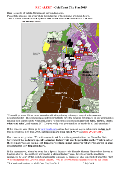
Simulation of the interannual variations of aerosols in China: role of

Atmos. Chem. Phys., 14, 9597–9612, 2014
www.atmos-chem-phys.net/14/9597/2014/
doi:10.5194/acp-14-9597-2014
© Author(s) 2014. CC Attribution 3.0 License.
Simulation of the interannual variations of aerosols in China:
role of variations in meteorological parameters
Q. Mu1,2 and H. Liao1
1 State
Key Laboratory of Atmospheric Boundary Layer Physics and Atmospheric Chemistry, Institute of Atmospheric
Physics, Chinese Academy of Sciences, Beijing, China
2 Graduate University of Chinese Academy of Sciences, Beijing, China
Correspondence to: H. Liao ([email protected])
Received: 18 March 2014 – Published in Atmos. Chem. Phys. Discuss.: 7 May 2014
Revised: 31 July 2014 – Accepted: 10 August 2014 – Published: 16 September 2014
Abstract. We used the nested grid version of the global
three-dimensional Goddard Earth Observing System chemical transport model (GEOS-Chem) to examine the interannual variations (IAVs) of aerosols over heavily polluted regions in China for years 2004–2012. The role of variations
in meteorological parameters was quantified by a simulation with fixed anthropogenic emissions at year 2006 levels and changes in meteorological parameters over 2004–
2012. Simulated PM2.5 (particles with a diameter of 2.5 µm
or less) aerosol concentrations exhibited large IAVs in North
China (NC; 32–42◦ N, 110–120◦ E), with regionally averaged absolute percent departure from the mean (APDM)
values of 17, 14, 14, and 11 % in December-JanuaryFebruary (DJF), March-April-May (MAM), June-JulyAugust (JJA), and September-October-November (SON), respectively. Over South China (SC; 22–32◦ N, 110–120◦ E),
the IAVs in PM2.5 were found to be the largest in JJA, with
the regional mean APDM values of 14 % in JJA and of about
9 % in other seasons. The concentrations of PM2.5 over the
Sichuan Basin (SCB; 27–33◦ N, 102–110◦ E) were simulated
to have the smallest IAVs among the polluted regions examined in this work, with APDM values of 8–9 % in all seasons.
All aerosol species (sulfate, nitrate, ammonium, black carbon, and organic carbon) were simulated to have the largest
IAVs over NC in DJF, corresponding to the large variations
in meteorological parameters over NC in this season. Process analyses were performed to identify the key meteorological parameters that determined the IAVs of different
aerosol species in different regions. While the variations in
temperature and specific humidity, which influenced the gasphase formation of sulfate, jointly determined the IAVs of
sulfate over NC in both DJF and JJA, wind (or convergence
of wind) in DJF and precipitation in JJA were the dominant
meteorological factors to influence IAVs of sulfate over SC
and the SCB. The IAVs in temperature and specific humidity
influenced gas-to-aerosol partitioning, which were the major factors that led to the IAVs of nitrate aerosol in China.
The IAVs in wind and precipitation were found to drive the
IAVs of organic carbon aerosol. We also compared the IAVs
of aerosols simulated with variations in meteorological parameters alone with those simulated with variations in anthropogenic emissions alone; the variations in meteorological fields were found to dominate the IAVs of aerosols in
northern and southern China over 2004–2012. Considering
that the IAVs in meteorological fields are mainly associated
with natural variability in the climate system, the IAVs in
aerosol concentrations driven by meteorological parameters
have important implications for the effectiveness of shortterm air quality control strategies in China.
1
Introduction
Aerosols are major air pollutants that have adverse effects
on human health, reduce atmospheric visibility, and influence global climate change. With the rapid economic development in China over the past decades, concentrations
of aerosols are now among the highest in the world (Fu et
al., 2008; Cao et al., 2012; Sun et al., 2013), driven mainly
by the increases in direct and precursor emissions (Streets
et al., 2003). Aerosol concentrations in China have variations on different timescales (Zhang et al., 2010a; Zhu et al.,
Published by Copernicus Publications on behalf of the European Geosciences Union.
9598
Q. Mu and H. Liao: Simulation of the interannual variations of aerosols in China
2012); we aim to understand interannual variations (IAVs) of
aerosols in this study. Understanding interannual variations
in aerosols driven by variations in meteorological parameters
is especially important for air pollution control. For example, the Action Plan for Air Pollution Prevention and Control
released by the State Council of China in 2013 aims to reduce the annual mean PM2.5 concentrations in the regions of
Beijing-Tianjin-Hebei, Yangtze Delta, and Pearl River delta
by 25, 20, and 15 % respectively, as the concentrations in
year 2017 are compared with those in 2012. The role of interannual variations in meteorological parameters needs to be
separated from the impact of the reductions in emissions in
these targeted reductions.
The IAVs of aerosols were usually quantified in previous studies by statistical variables such as standard deviation (SD), relative standard deviation (RSD), mean absolute
deviation (MAD), and absolute percent departure from the
mean (APDM), which are defined as
s
2
1 Xn
1 Xn
C
−
C
,
(1)
SD =
i
i=1
i=1 i
n
n
X
1
n
C ,
RSD = 100 % × SD/
i=1 i
n
(2)
1 Xn
1 Xn Ci −
Ci ,
MAD =
i=1
i=1
n
n
(3)
X
1
n
APDM = 100 % × MAD/
C ,
i=1 i
n
(4)
where Ci is aerosol concentration of year i, and n is the number of years examined. Therefore SD and MAD represent the
absolute IAVs in aerosol concentration, and RSD and APDM
represent the IAVs relative to the average concentration over
the n years.
Large IAVs of aerosols have been reported in previous
studies for different aerosol species in different regions. Mahowald et al. (2003) showed that annual mean mineral dust
concentrations measured at 10 sites in the United States over
1979–2000 had RSD values of 57–101 %. Habib et al. (2006)
found by using the Total Ozone Mapping Spectrometer absorbing aerosol index data sets that the absorbing aerosol
column burdens averaged over April–May of 1981–1992 exhibited a RSD of 16–30 % in different regions of India. Alston et al. (2012) showed by using ground-based measurements at 41 sites in the southeastern United States (29 sites of
PM2.5 measurements provided by Environmental Protection
Agency and 12 sites by Georgia Dept. of Natural Resources)
that monthly mean PM2.5 concentrations in that region had
APDM values of 5–10 % over 2000–2009. They also showed
by using three sets of aerosol optical depth (AOD) from Moderate Resolution Imaging Spectroradiometer (MODIS) Terra,
Atmos. Chem. Phys., 14, 9597–9612, 2014
Multi-angle Imaging Spectroradiometer Terra, and MODIS
Aqua that monthly mean AOD in the southeastern United
States had RSD values of 15–25 % over 2000–2009.
Observations and modeling studies have also shown that
aerosols in China have large IAVs. Qu et al. (2010) reconstructed PM10 aerosol concentrations at 86 Chinese cities
using records of air pollution index from summer 2000
to winter 2006, and reported that seasonal-median PM10
levels exhibited APDM values of 15–35 % in those cities.
Yang et al. (2011) collected weekly samples of carbonaceous
aerosols over 2005–2008 at two sites in Beijing and reported
that year-to-year changes in emission and meteorology altered annual-average fine organic carbon (OC) concentrations at the rural site in Beijing by as much as 27 % over
the observational time period.
The IAVs of aerosols are influenced by both emissions and
meteorology. Meteorological parameters influence aerosol
concentrations through altering emissions, chemical reactions, transport, and deposition. For example, increases in
temperature enhance chemical production of sulfate in the
atmosphere (Aw and Kleeman, 2003; Dawson et al., 2007;
Kleeman, 2008) and decrease nitrate aerosol formation (Bellouin et al., 2011; Liao et al., 2006; Pye et al., 2009; Racherla
and Adams, 2006). Aerosol concentrations decrease with increasing precipitation as wet deposition provides the main
aerosol sink (Balkanski et al., 1993; Dawson et al., 2007),
and changes in ventilation (wind speed, mixing depth) have
large impacts on aerosols since aerosols are mainly influenced by local meteorological conditions. Tai et al. (2010)
found that daily variation in meteorology as described by the
multiple linear regression could explain up to 50 % of PM2.5
variability based on an 11-year (1998–2008) observational
record over the contiguous United States, with temperature,
relative humidity, precipitation, and circulation all being important predictors.
Since concentrations of chemical species are the net results
from comprehensive physical and chemical processes, the integrated process rates (IPR) (Im et al., 2011) have been used
to identify the dominant processes (such as horizontal and
vertical transport, emissions of primary species, gas-phase
chemistry, dry deposition, cloud processes, and aerosol processes) that influence the concentrations of chemical species
in the Community Multi-scale Air Quality model (CMAQ)
for episodic events (Jose et al., 2002; Goncalves et al., 2009)
as well as for yearly (Zhang et al., 2009) to decadal simulations (Civerolo et al., 2010). The IPR analyses in these studies ranked the roles of different processes in the formation
and fate of a chemical species. For example, the horizontal flows and gas-phase chemical reactions in the morning
and the vertical flows in the afternoon were found to be the
main factors in the formation of surface O3 during a photochemical pollution episode in the coastal area of southwestern Europe in summer (Goncalves et al., 2009). Recently,
a similar process analysis scheme was implemented within
the Weather Research and Forecasting model coupled with
www.atmos-chem-phys.net/14/9597/2014/
Q. Mu and H. Liao: Simulation of the interannual variations of aerosols in China
Chemistry (WRF Chem) to understand the key photochemical and physical processes for the formation of O3 (Jiang et
al., 2012) and PM10 (Jiang et al., 2013).
The scientific goals of this work are (1) to quantify the IAVs in surface-layer aerosol concentrations in
China resulted from the variations in meteorological conditions during the 2004–2012 period, using the global threedimensional chemical transport model GEOS-Chem (Goddard Earth Observing System chemical transport model), and
(2) to identify the key meteorological parameters that influenced the IAVs of aerosols in different polluted regions of
China by the IPR analyses. Section 2 describes the model,
emissions, and numerical experiments. Section 3 presents
simulated distributions of aerosols and IAVs in concentrations of different aerosol species in China averaged over
2004–2012. The key meteorological parameters that influenced IAVs of aerosols are examined by IPR in Sect. 4. Section 5 discusses the impacts of anthropogenic and natural
emissions on IAVs of aerosols in China.
2
2.1
Model description and numerical experiments
GEOS-Chem Model
We simulated aerosols using the global chemical transport model GEOS-Chem (version 9-01-02) driven by the
GEOS-5 assimilated meteorological fields from the Goddard Earth Observing System of the NASA Global Modeling and Assimilation Office. We used the nested-grid capability of the GEOS-Chem model over East Asia (11◦ S–55◦ N,
70–150◦ E) with a horizontal resolution of 0.5◦ latitude by
0.667◦ longitude and 47 vertical layers up to 0.01 hPa (Chen
et al., 2009). Chemical boundary conditions were from the
global simulations performed at 4◦ ×5◦ horizontal resolution.
The GEOS-Chem model has fully coupled O3 –NOx –
hydrocarbon chemistry and aerosols including sulfate
−
+
(SO2−
4 ), nitrate (NO3 ), ammonium (NH4 ) (Park et al., 2004;
Pye et al., 2009), OC and BC (black carbon; Park et al.,
2003), sea salt (Alexander et al., 2005), and mineral dust
(Fairlie et al., 2007). The gas–aerosol partitioning of nitric
acid and ammonia is calculated using the ISORROPIA II
thermodynamic equilibrium model (Fountoukis and Nenes,
2007). Wet deposition of soluble aerosols and gases follows
the scheme of Liu et al. (2001) and dry deposition follows a
standard resistance-in-series model of Wesely (1989). We do
not examine IAVs of mineral dust and sea salt aerosols in this
study, because sea salt aerosol is not a major aerosol component in China based on measurements (Ye et al., 2003; Duan
et al., 2006) and mineral dust aerosol simulation has very
large uncertainties (Fairlie et al., 2007, 2010).
Considering the large uncertainties in chemistry schemes
of secondary organic aerosol (SOA), SOA in our simulations
was assumed to be the 10 % carbon yield of OC from biowww.atmos-chem-phys.net/14/9597/2014/
9599
genic terpenes (Park et al., 2003) and 2 % carbon yield of
OC from biogenic isoprene (van Donkelaar et al., 2007).
2.2
Emissions
Global emissions of aerosol precursors and aerosols in the
GEOS-Chem model generally follow Park et al. (2003) and
Park et al. (2004). Anthropogenic emissions of NOx , SO2 ,
BC, and OC (including emissions from power, industry, residential, and transportation sources) in the Asian domain are
overwritten by David Streets’ 2006 emission inventory (http:
//mic.greenresource.cn/intex-b2006) (Zhang et al., 2009) in
this work. Estimates of NH3 emissions in China showed
large uncertainties in previous studies (Streets et al., 2003;
Kim et al., 2006; Zhang et al., 2010b; Huang et al., 2011,
2012). We used in our simulations the most recent estimate of NH3 emissions in China by Huang et al. (2012),
which was 9.8 Tg yr−1 , instead of 13.5 Tg yr−1 from Streets
et al. (2003). Monthly variations in SO2 , NOx , and NH3
follow those in Wang et al. (2013). Table 1 summarizes
year 2006 annual emissions of NOx , SO2 , NH3 , OC, and
BC in Asia (70–150◦ E, 11◦ S–55◦ N) and eastern China (98–
130◦ E, 20–55◦ N).
Natural NOx emissions from lightning were described by
Sauvage et al. (2007) and Murray et al. (2012), and those
from soil were described by Yienger and Levy (1995). Natural NH3 emissions from soil, vegetation, and the oceans
were from the Global Emissions Inventory Activity inventory
(Bouwman et al., 1997). Biomass burning emissions were
from the monthly Global Fire Emissions Database-v2 inventory (van der Werf et al., 2006). Biogenic VOC (volatile organic compounds) emissions were calculated from the Model
of Emissions of Gases and Aerosols from Nature (Guenther
et al., 2006).
2.3
Numerical experiments
To quantify IAVs of aerosols over 2004–2012, we performed
the following simulations of aerosols in China using the
GEOS-Chem model driven by the GEOS-5 meteorological
fields:
1. ANNmet: the simulation to examine how the IAVs of
aerosols were influenced by variations in meteorological parameters. Meteorological fields, natural emissions, and biomass burning emissions were allowed to
vary from 2004 to 2012, while anthropogenic emissions
were kept at the year 2006 values.
2. ANNmet_ATM: sensitivity simulation for 2004–2012
to examine the sensitivity of IAVs of aerosols to variations in atmospheric conditions alone. All natural emissions (such as soil NOx , lightning NOx as well as biogenic sources) that were sensitive to meteorological
parameters were turned off. Anthropogenic emissions
were kept at the year 2006 values. Meteorological fields
Atmos. Chem. Phys., 14, 9597–9612, 2014
9600
Q. Mu and H. Liao: Simulation of the interannual variations of aerosols in China
Table 1. Summary of annual emissions of aerosols and aerosol precursors in Asia (70–150◦ E, 11◦ S–55◦ N) and eastern China (98–
130◦ E, 20–55◦ N).
Species
Asia
Eastern
China
0.08
10.6
1.09
0.02
0.35
1.16
0.88
14.18
0.02
6.38
0.14
< 0.01
0.12
0.28
0.27
7.21
0.01
23.85
0.36
< 0.01
3.99
0.48
28.69
< 0.01
15.98
0.04
< 0.01
0.07
0.05
16.14
14.18
2.33
0.82
0.8
18.13
7.26
0.49
0.11
0.3
8.16
1.54
4.62
3.47
2.5
12.13
1.03
0.67
1.44
0.55
3.69
1.52
0.55
0.92
2.99
0.96
0.05
0.39
1.4
NOx (Tg N yr−1 )
Aircraft
Anthropogenic
Biomass burning
Biofuel
Fertilizer
Lightning
Soil
Total
Figure 1. Polluted regions examined in this study, including North
China (NC, 32–42◦ N, 110–120◦ E), South China (SC, 22–32◦ N,
110–120◦ E), and the Sichuan Basin (SCB, 27–33◦ N, 102–110◦ E).
SO2 (Tg S yr−1 )
Aircraft
Anthropogenic
Biomass burning
Biofuel
Volcanoes
Ship
Total
and biomass burning emissions were allowed to vary
from 2004 to 2012.
3. ANNemis: the simulation to examine how the IAVs of
aerosols were influenced by variations in anthropogenic
emissions. Anthropogenic and biomass burning emissions were allowed to vary from 2004 to 2012. Meteorological parameters and hence natural emissions were
kept at the year 2006 values.
NH3 (Tg N yr−1 )
Anthropogenic
Natural
Biomass burning
Biofuel
Total
4. ANNall: simulation of aerosols for years 2004–
2012 with yearly varying meteorological parameters,
biomass, natural and anthropogenic emissions. The
IAVs in anthropogenic emissions over 2004–2012 were
obtained by using scaling factors; the annual scaling
factors for NOx were taken from Zhang et al. (2012)
and those for SO2 , OC, and BC were taken from Lu et
al. (2011).
In ANNmet, the IAVs in meteorological fields influenced
aerosol concentrations in two ways. First, changes in meteorological parameters influenced chemical reactions, transport, and deposition of aerosols. Second, precursor emissions
from natural sources varied with meteorological fields. We
performed one sensitivity simulation ANNmet_ATM with
natural emissions turned off. The differences between ANNmet and ANNmet_ATM represent the differences in IAVs
with and without natural emissions. Biomass burning emissions were partly anthropogenic and partly natural, which
were allowed to vary over 2004–2012 in all the simulations.
A comparison of ANNmet and ANNemis tells us the relative
importance of variations in meteorological parameters and
anthropogenic emissions in IAVs of aerosols.
The presentations of the IAVs of aerosols will be focused on three polluted regions in China, NC (32–42◦ N,
110–120◦ E), SC (22–32◦ N, 110–120◦ E), and the SCB (27–
33◦ N, 102–110◦ E), as defined in Fig. 1.
Atmos. Chem. Phys., 14, 9597–9612, 2014
OC (Tg C yr−1 )
Anthropogenic
Biomass burning
Biofuel
Biogenic
Total
BC (Tg C yr−1 )
Anthropogenic
Biomass burning
Biofuel
Total
3
3.1
Simulated IAVs of aerosols resulted from IAVs of
meteorological parameters alone
Simulated distributions of aerosol concentrations
Figure 2 shows simulated seasonal mean surface-layer concentrations of sulfate, nitrate, ammonium, OC, BC, and
PM2.5 (sum of sulfate, nitrate, ammonium, OC, and BC) averaged over 2004–2012 of simulation ANNmet. The simulated aerosol concentrations were high over polluted eastern
www.atmos-chem-phys.net/14/9597/2014/
Q. Mu and H. Liao: Simulation of the interannual variations of aerosols in China
Figure 2. Simulated seasonal mean surface-layer concentrations
(µg m−3 ) of sulfate, nitrate, ammonium, OC, BC, and PM2.5 in ANNmet averaged over 2004–2012.
China throughout the year. Sulfate concentrations in NC
were 15–20 µg m−3 in June-July-August (JJA) with the
strong photochemistry in that season, and the concentrations
over SC showed small values of 3–10 µg m−3 in JJA as a
result of the large precipitation associated with the summer monsoon. The maximum sulfate concentrations of 25–
30 µg m−3 were simulated over SCB in December-JanuaryFebruary (DJF), as a result of the large SO2 emissions from
winter heating. Our simulated seasonal variations in sulfate
concentrations agree well with those in Wang et al. (2013).
Simulated nitrate concentrations over NC were in the
range of 15–40 µg m−3 throughout the year, with maximum
concentrations of about 40 µg m−3 in DJF. High NOx emissions and low temperatures favored nitrate formation in DJF.
Nitrate concentrations showed values of 5–15 µg m−3 over
SC and SCB in JJA when temperatures were the highest.
Simulated ammonium concentrations were in the range of 5–
20 µg m−3 over NC, SC, and SCB, with seasonal variations
in these regions following those of nitrate.
The simulated distributions of OC and BC were similar
to those of their emissions, with the highest values in NC.
Simulated OC and BC concentrations were high in DJF and
September-October-November (SON) and low in MarchApril-May (MAM) and JJA, owing to the seasonal variations
in precipitation.
Simulated PM2.5 concentrations were in the range of 70–
90 µg m−3 in NC throughout the year, which were generally
higher than the concentrations in SC and SCB. In the surface
layer, nitrate was predicted to be the most abundant aerosol
species over eastern China, followed by sulfate, ammonium,
www.atmos-chem-phys.net/14/9597/2014/
9601
Figure 3. MAD (µg m−3 ) of surface-layer concentrations of sulfate,
nitrate, ammonium, OC, BC, and PM2.5 simulated in ANNmet for
years 2004–2012.
OC, and BC. Wang et al. (2013) reported that high nitrate in
the GEOS-Chem model is likely caused by the overestimate
of NH3 emissions; and Kharol et al. (2013) demonstrated that
the persistent nitrate in GEOS-Chem in China is, overall, as
much linked to high NOx emissions as it is to high NH3 emissions.
3.2
Simulated IAVs of aerosols
Figures 3 and 4 show, respectively, the MAD and APDM values of seasonal mean surface-layer concentrations of sulfate,
nitrate, ammonium, OC, BC, and PM2.5 simulated in ANNmet. We also present the domain-averaged values of MAD
and APDM for NC, SC, and SCB in Tables 2 and 3.
The MAD and APDM values of sulfate, nitrate, and ammonium from ANNmet indicated that concentrations of these
species in NC had larger IAVs than those in SC (Tables 2,
3). Over NC, SC, and SCB, sulfate aerosol showed regional
mean APDM values of 10–24 %. The largest IAVs of sulfate were found over NC in DJF, with APDM values exceeding 24 %. These IAVs were significant, considering that these
were averages over 2004–2012; year by year variations can
be larger than the averages reported here. Our simulated IAV
of sulfate was close to the IAV of 14–20 % reported by Gong
et al. (2010) for sulfate at the Canadian high Arctic.
The MAD and APDM values obtained in simulation ANNmet showed that nitrate concentrations also had large IAVs
(Tables 2, 3). The APDM values were 13–18 % over NC
where nitrate concentrations were the highest. The APDM
values of nitrate in NC did not show large variations with season, which were larger than the APDM values of sulfate in
Atmos. Chem. Phys., 14, 9597–9612, 2014
Q. Mu and H. Liao: Simulation of the interannual variations of aerosols in China
9602
ANNemis
24.6
20.0
18.2
13.1
13.9
17.9
ANNall
17.0
15.6
15.2
10.7
8.7
13.8
ANNmet
16.7
15.7
15.1
8.7
8.7
13.8
ANNmet_ATM
4.1
8.2
4.6
5.0
2.9
4.7
ANNemis
18.2
19.2
17.1
11.3
10.4
15.8
ANNall
ANNmet_ATM
0.5
1.0
0.2
0.2
0.2
1.3
ANNemis
1.7
1.7
0.8
0.5
0.2
4.1
2.0
2.6
1.2
0.6
0.3
6.4
ANNall
1.0
0.7
0.5
0.2
0.1
2.0
1.2
1.2
0.7
0.3
0.1
3.1
1.3
1.8
1.0
0.3
0.1
4.4
ANNmet
1.0
0.7
0.5
0.2
0.1
2.0
1.2
1.2
0.7
0.2
0.1
3.0
1.3
1.8
0.9
0.3
0.1
4.2
ANNmet_ATM
0.7
0.9
0.5
0.1
0.1
2.1
0.4
1.4
0.5
0.1
0.1
2.1
0.5
1.5
0.4
0.1
0.1
2.1
ANNemis
1.3
1.1
0.7
0.3
0.1
3.1
1.2
2.0
0.9
0.3
0.1
4.2
1.3
2.5
1.1
0.3
0.2
5.1
ANNall
NC
SC
SCB
NC
SC
SCB
ANNmet_ATM
4.4
11.1
5.4
5.1
2.7
5.3
ANNemis
14.6
19.6
15.6
8.5
9.6
14.5
ANNall
13.7
13.0
11.7
7.7
7.5
10.7
ANNmet
13.6
13.2
11.7
7.6
7.5
10.8
ANNmet_ATM
4.5
10.8
5.9
5.1
2.5
5.7
4.3
8.0
3.4
5.1
3.0
3.6
ANNemis
12.1
16.6
13.6
7.6
7.9
10.7
17.3
15.1
13.4
8.5
8.9
12.5
ANNall
SON
ANNmet
14.7
17.4
14.8
8.2
8.3
13.7
10.5
11.9
9.4
6.8
6.9
8.6
JJA
14.7
17.0
14.9
8.3
8.2
13.7
10.6
12.2
9.5
7.2
6.9
8.6
13.7
14.8
11.1
6.2
7.7
10.5
17.6
24.5
19.8
9.3
10.2
17.1
7.3
10.9
6.9
5.1
2.8
6.8
ANNall
6.2
14.7
9.6
5.1
2.1
8.4
ANNemis
1.6
2.3
1.0
0.3
0.2
4.8
15.1
16.7
15.4
8.8
8.2
13.4
ANNmet_ATM
0.5
1.5
0.4
0.1
0.1
1.9
1.2
1.9
0.8
0.3
0.1
3.8
10.6
9.8
8.5
5.6
5.8
7.9
ANNmet
1.5
2.0
1.0
0.3
0.2
4.8
0.5
1.4
0.5
0.1
0.1
2.3
1.5
1.3
0.7
0.2
0.1
3.4
10.7
10.5
8.7
5.6
5.8
8.0
ANNall
1.5
2.1
1.0
0.3
0.2
4.9
1.1
1.3
0.7
0.2
0.1
3.1
0.9
0.9
0.5
0.1
0.1
2.3
15.0
21.6
16.2
6.9
8.0
14.0
ANNemis
1.5
3.0
1.3
0.3
0.2
5.7
1.1
1.3
0.7
0.3
0.1
3.1
1.2
0.8
0.6
0.2
0.1
2.5
8.9
17.0
10.8
5.1
2.5
9.2
ANNmet_ATM
0.4
1.9
0.5
0.1
0.1
2.6
0.9
1.8
0.8
0.2
0.1
3.6
1.3
0.8
0.6
0.2
0.1
2.5
10.2
11.3
10.0
5.8
5.4
8.8
ANNmet
1.4
2.3
1.1
0.3
0.1
4.9
0.3
1.3
0.4
0.1
0.1
2.0
1.1
1.3
0.7
0.2
0.1
3.2
10.8
12.9
10.8
5.8
5.4
9.2
1.4
2.4
1.1
0.3
0.1
5.0
0.9
1.2
0.6
0.2
0.1
2.8
0.7
0.8
0.5
0.1
0.1
2.0
SON
0.9
1.2
0.6
0.2
0.1
2.8
1.0
0.8
0.5
0.2
0.1
2.4
15.7
17.7
16.1
9.2
8.3
13.8
Table 3. Simulated APDM values (%) of aerosols in ANNmet, ANNmet_ATM, ANNemis, and ANNall.
ANNmet_ATM
4.2
5.0
1.9
5.1
3.2
2.5
MAM
ANNmet
23.8
18.3
17.1
12.1
12.1
16.9
DJF
23.6
18.2
17.0
12.1
12.0
16.9
Species
SO42−
NO3−
NH4+
OC
BC
PM2.5
14.1
18.0
14.5
10.4
9.8
13.5
13.8
15.9
12.7
8.2
8.1
11.8
4.6
11.0
6.4
5.0
2.5
6.2
7.4
11.9
7.9
5.1
2.8
7.4
11.6
11.5
10.3
7.4
7.2
9.5
9.6
9.3
8.2
5.5
5.4
7.5
11.8
11.7
10.5
10.3
7.7
9.7
10.1
9.3
8.5
6.6
5.3
7.6
15.5
13.0
10.9
12.5
10.5
10.6
16.6
14.3
10.3
8.9
9.5
10.5
4.4
5.9
2.9
5.0
2.8
3.4
5.4
6.5
3.1
5.0
3.0
4.1
14.1
11.5
9.2
7.6
7.8
8.8
14.2
11.5
9.0
6.8
7.4
8.8
13.9
11.5
9.3
11.9
8.6
9.2
14.4
11.4
9.0
7.3
7.4
8.8
SO42−
NO3−
NH4+
OC
BC
PM2.5
SO42−
NO3−
NH4+
OC
BC
PM2.5
ANNmet
2.1
2.3
1.2
0.5
0.3
6.2
0.5
0.8
0.2
0.1
0.1
1.4
2.0
1.5
0.7
0.4
0.2
3.7
JJA
0.9
0.8
0.5
0.2
0.1
2.3
Table 2. Simulated MAD values (µg m−3 ) of aerosols in ANNmet, ANNmet_ATM, ANNemis, and ANNall.
2.0
2.3
1.2
0.5
0.3
6.1
1.8
1.4
0.8
0.3
0.2
3.6
0.8
0.7
0.2
0.1
0.1
1.7
MAM
SO42−
NO3−
NH4+
OC
BC
PM2.5
1.7
1.4
0.8
0.5
0.2
3.7
1.8
1.2
0.6
0.3
0.1
3.1
DJF
SO42−
NO3−
NH4+
OC
BC
PM2.5
1.8
1.2
0.6
0.3
0.2
3.1
Species
SO42−
NO3−
NH4+
OC
BC
PM2.5
www.atmos-chem-phys.net/14/9597/2014/
Atmos. Chem. Phys., 14, 9597–9612, 2014
Q. Mu and H. Liao: Simulation of the interannual variations of aerosols in China
Figure 4. APDM (%) of surface-layer concentrations of sulfate, nitrate, ammonium, OC, BC, and PM2.5 simulated in ANNmet for
years 2004–2012.
JJA but smaller than those of sulfate in DJF. The distribution
and magnitude of the APDM values of ammonium generally
followed those of nitrate over polluted eastern China.
The spatial pattern of either MAD or APDM of OC was
similar to that of BC in all seasons. OC exhibited seasonal
mean APDM values of 6–12 % in polluted NC, SC, and SCB
throughout the year. Because BC is a chemically inert tracer,
the IAVs in BC obtained in ANNmet were caused by the variations in transport and deposition. The APDM values of BC
were about the same as those of OC, except that the APDM
values of BC were smaller in NC in MAM and in SC in DJF,
MAM, and JJA.
The IAVs of PM2.5 concentrations were the largest in NC;
the regional mean APDM values were 17, 14, 14, and 11 % in
DJF, MAM, JJA, and SON (Table 3), respectively. Over SC,
the maximum APDM value of 14 % was found in JJA and
the highest APDM values were about 9 % in the other seasons (Table 3). Over SCB, PM2.5 showed the smallest IAVs
among all regions, with APDM values of 8–9 % in all seasons.
3.3
Comparisons of simulated IAVs of aerosols with
measurements
Simulated concentrations of sulfate, nitrate, and ammonium
aerosols in China have been evaluated in the study of Wang
et al. (2013) and those of carbonaceous aerosols in China
have been evaluated by Fu et al. (2012), both of which used
the same one-way nested-grid capability of the GEOS-Chem.
www.atmos-chem-phys.net/14/9597/2014/
9603
Wang et al. (2013) found that simulated concentrations of
sulfate, nitrate and ammonium at 22 sites in East Asia exhibited annual mean biases of −10, +31, and +35 %, respectively; and Fu et al. (2012) showed that the simulated annual
mean concentrations of BC and OC averaged over rural and
background sites were underestimated by 56 and 76 %, respectively.
For the purpose of this study, we evaluated the model’s
performance in simulating the IAVs of aerosols by comparing simulated AODs with satellite measurements, because of the lack of long-term ground-based measurements
in China (Chan and Yao, 2008). The Level 3 MODIS/Terra
monthly products (MOD08_M3; http://ladsweb.nascom.
nasa.gov/) with 1◦ ×1◦ equal-angle global grid were obtained
from NASA’s LAADS (Level 1 and Atmosphere Archive and
Distribution System). Collections 5 and 5.1 contain the time
series of AODs from March 2000 to the present. We used
AODs at the 550 nm wavelength, which incorporated only
the highest quality retrievals. Over East Asia, the MODIS
measurements have been well validated through many studies (Chin et al., 2004; Park et al., 2011). In the GEOS-Chem
model, the AODs of sulfate, nitrate, ammonium, OC, BC, sea
salt, and dust aerosols were calculated based on aerosol mass
concentration, extinction efficiency, effective radius, particle mass density, and the assumed aerosol size distribution
(Drury et al., 2010). The hygroscopic growth of each aerosol
species with relative humidity was accounted for, using the
hygroscopic growth factors listed in Martin et al. (2003).
We compared simulated and observed IAVs in AODs for
the cities of Beijing (39.5◦ N, 116.2◦ E), Changsha (28.1◦ N,
112.6◦ E) and Chengdu (30.7◦ N, 104.0◦ E) (Fig. 5), which
were chosen to represent the model performance in the NC,
SC and SCB regions, respectively. The correlation coefficients between observed and modeled monthly mean AODs
from ANNmet simulations were 0.83, 0.34, and 0.13 for
Beijing, Changsha, and Chengdu, respectively. The large
correlation coefficient for Beijing indicates that the model
was able to capture to some extent the observed IAVs in
NC. The small correlation coefficients in Chengdu can be
explained in part by the complex topography and satellite
limitations such as cloud contamination (Xia et al., 2004).
Note that in simulation ANNmet, simulated AODs correlated well with the simulated column burdens and surfacelayer concentrations of PM2.5 ; the correlation coefficients between simulated monthly mean AODs and column burdens
(surface-layer concentrations) of PM2.5 were 0.95 (0.81),
0.94 (0.81), and 0.91 (0.77) over Beijing, Changsha, and
Chengdu, respectively. The IAVs of observed AODs agreed
fairly well with the IAVs of surface-layer aerosol concentrations. For example, the seasonal mean APDM values of
observed AODs were 18 (DJF), 15 (MAM), 24 (JJA), and
16 % (SON) for Beijing, close to the seasonal mean APDM
values of surface-layer PM2.5 shown in Fig. 4.
Atmos. Chem. Phys., 14, 9597–9612, 2014
9604
Q. Mu and H. Liao: Simulation of the interannual variations of aerosols in China
Figure 5. MODIS AOD (black line, left axis), simulated AOD in ANNall (red dotted line, left axis), simulated AOD in ANNmet (red line,
left axis), simulated surface-layer PM2.5 concentrations in ANNmet (green line, µg m−3 , right axis), and simulated column burden of PM2.5
in ANNmet (blue line, mg m−2 , right axis) over polluted cities of (a) Beijing, (b) Changsha, and (c) Chengdu.
4
4.1
Understanding the IAVs of aerosols by process
analyses
IAVs of meteorological parameters
Figure 6 shows seasonal mean temperature, specific humidity, precipitation, 850 hPa zonal and meridional winds for
DJF and JJA. All these meteorological fields were averaged
over years 2004–2012. Over central and eastern China, temperature, specific humidity and precipitation generally exhibited much larger values in JJA than in DJF. At 850 hPa, strong
westerlies were found in NC in DJF, and prevailing southerlies occurred in JJA, reflecting the typical features of winds
in China.
Figures 7 and 8 show, respectively, the MAD and APDM
values of surface-layer temperature, specific humidity, and
precipitation for DJF and JJA. The APDM values of temperature in DJF were generally larger than those in JJA. Piao et
al. (2003) also showed that the largest IAV of temperature in
eastern China was in winter (December and February) based
on the reanalyzed temperatures over 1982–1999. Specific humidity showed APDM values of 6–20 % in DJF and of 2–
8 % in JJA over central and eastern China. For precipitation,
APDM values of 20–80 % and 10–30 % were calculated in
Atmos. Chem. Phys., 14, 9597–9612, 2014
DJF and JJA, respectively, and the APDM values of precipitation were larger in NC than in SC, which agreed with those
reported in Qian and Lin (2005). The variations in temperature and specific humidity can influence chemical reactions
of sulfate, nitrate and ammonium, while those in precipitation are important for wet deposition of all aerosol species.
The relatively large APDM values of these meteorological
parameters in DJF suggested large IAVs of aerosols in this
season.
4.2
Process analyses
The concentrations of aerosols are determined by emissions,
chemical reactions, transport, and deposition. Therefore, the
IAVs of aerosols are influenced by the IAV of each of these
processes. The weighted contribution of each process to IAV
of an aerosol is estimated here using
Xn
% PCi =MADi /
MADi ,
(5)
i
where n is the number of processes considered, MADi is the
MAD value of process i and % PCi is the relative contribution of process i to the sum of the contributions from all processes (Im et al., 2011). Once the most important processes
are selected from this approach, meteorological variables to
www.atmos-chem-phys.net/14/9597/2014/
Q. Mu and H. Liao: Simulation of the interannual variations of aerosols in China
9605
Figure 7. The MAD values of surface air temperature (K), specific humidity (g kg−1 ) and precipitation (mm d−1 ) in DJF and JJA
based on the GEOS-5 assimilated meteorological fields of 2004–
2012.
Figure 6. Seasonal mean surface air temperature (K), specific
humidity (g kg−1 ), precipitation (mm d−1 ), zonal and meridional
wind at 850 hPa (m s−1 ) in DJF and JJA. Winds that were eastward or northward were positive, and those that were westward
and southward were negative. Meteorological fields were from the
GEOS-5 assimilated meteorological data and were averaged over
2004–2012.
which the processes are sensitive to are classified as the key
meteorological parameters that lead to IAV of the aerosol.
Since we aimed to examine the IAVs in surface-layer aerosol
concentrations, our process analyses for an aerosol species
were performed for each region (NC, SC, or SCB) from the
surface to 1 km altitude. For an aerosol species, the budget
(mass flux from each process) was constructed for the selected region considering the mass balance of this aerosol.
Chemical production and removal, transport, as well as wet
and dry deposition of the aerosol were diagnosed at every
time step and summed over each season in simulation ANNmet.
4.2.1
Sulfate
Processes that influence the IAVs of sulfate concentrations
include anthropogenic emissions, formation pathways (gaswww.atmos-chem-phys.net/14/9597/2014/
Figure 8. The APDM values ( %) of surface air temperature, specific humidity, and precipitation in DJF and JJA based on the
GEOS-5 assimilated meteorological fields of 2004–2012.
phase oxidation of SO2 by OH, and in-cloud oxidation of
SO2 by ozone and hydrogen peroxide), mass fluxes through
the four lateral boundaries and the upper boundary at 1 km,
wet and dry deposition. On the basis of simulation ANNmet, Fig. 9 shows the mass fluxes and APDM values and
Fig. 10 shows the MAD values and relative contributions of
individual atmospheric processes to sulfate concentrations in
Atmos. Chem. Phys., 14, 9597–9612, 2014
9606
Q. Mu and H. Liao: Simulation of the interannual variations of aerosols in China
different regions for DJF and JJA. Transport fluxes were calculated at the boundaries while other sources and sinks were
the sums over the grid cells of the region under 1 km.
With respect to the sulfate budget over NC in DJF, vertical flux through the top side and gas-phase sulfate formation
by reaction of SO2 with OH had the largest values of 0.041
and 0.019 Tg S season−1 , respectively (Fig. 9a). Among the
four horizontal fluxes through the lateral boundaries of NC,
the flux through the south boundary had the largest value of
0.017 Tg S season−1 , while that through the west boundary
had the smallest value of 0.003 Tg S season−1 . The in-cloud
reactions of SO2 with O3 and H2 O2 contributed relatively little to sulfate formation, by 0.005 and 0.004 Tg S season−1 ,
respectively. Wet deposition was 0.006 Tg S season−1 and
dry deposition was the smallest flux. Figure 10 shows that
gas-phase oxidation of SO2 by OH was the most important
process that contributed to the IAV of sulfate, with a relative
contribution of 30 %, followed by the vertical flux through
the top side (18 %). The relative contributions of horizontal fluxes through the lateral boundaries were in the range
of 3–11 %. Each of the aqueous-phase oxidations of SO2 by
O3 and H2 O2 accounted for 6 % of the IAV of sulfate. The
relative contribution by wet deposition was 8 % and that by
dry deposition was 0.4 % (Fig. 10a). In JJA, the gas-phase
formation of sulfate increased to 0.039 Tg S season−1 with a
relative contribution of 57 %, making it the only process that
determined the IAV of sulfate concentration over NC in this
season. Since gas-phase oxidation of SO2 is sensitive to temperature and humidity (Yao et al., 2002; Zhang et al., 2012),
we conclude that the variations in temperature and specific
humidity were the key factors that drove the IAV of sulfate
over NC. The relatively high MAD values of temperature in
NC in both DJF and JJA (Fig. 7) as well as the large MAD
values of specific humidity over NC in JJA (Fig. 7) support
the above conclusion.
Similar analyses were performed for sulfate in SC. In
DJF, the gas-phase formation of sulfate and wet deposition were the dominant source and sink of sulfate in this
region (Fig. 9b). The vertical flux, flux through the south
boundary, and wet deposition had the largest contributions to
IAV of sulfate with relative contributions of 24, 18, and 15 %,
respectively, indicating that wind and precipitation were the
main meteorological factors that determined the IAV of sulfate concentration over SC in DJF. In JJA, sulfate formation from the reaction of SO2 with OH had a large value of
0.030 Tg S season−1 , but this process had a very low APDM
value of 6 % (Fig. 9b). Figure 10b showed that wet deposition
and in-cloud oxidation of SO2 by H2 O2 were the prevailing
processes that contributed, respectively, 20 and 18 % to the
IAV of sulfate concentration in SC. These two processes corresponded well with the high MAD values of precipitation in
JJA as shown in Fig. 7.
With respect to the sulfate budget over the SCB in DJF,
vertical flux through the top side, wet deposition, and gasphase formation of sulfate had the largest values of 0.050,
Atmos. Chem. Phys., 14, 9597–9612, 2014
(a)
DJF
JJA
90 80 70 60 50 40 30 20 10 0 -10 -20 -30 -40 -50 -60 -70 -80 -90
North boundary flux
South boundary flux
East boundary flux
West boundary flux
Vertical flux
Wet deposition
Dry deposition
In cloud SO2+O3
In cloud SO2+H2O2
SO4 gas formation
Anthropogenic emission
-0.05 -0.04 -0.03 -0.02 -0.01 0.00 0.01 0.02 0.03 0.04 0.05
90 80 70 60 50 40 30 20 10 0 -10 -20 -30 -40 -50 -60 -70 -80 -90
(b)
North boundary flux
South boundary flux
East boundary flux
West boundary flux
Vertical flux
Wet deposition
Dry deposition
In cloud SO2+O3
In cloud SO2+H2O2
SO4 gas formation
Anthropogenic emission
-0.05 -0.04 -0.03 -0.02 -0.01 0.00 0.01 0.02 0.03 0.04 0.05
90 80 70 60 50 40 30 20 10 0 -10 -20 -30 -40 -50 -60 -70 -80 -90
(c)
North boundary flux
South boundary flux
East boundary flux
West boundary flux
Vertical flux
Wet deposition
Dry deposition
In cloud SO2+O3
In cloud SO2+H2O2
SO4 gas formation
Anthropogenic emission
-0.05 -0.04 -0.03 -0.02 -0.01 0.00 0.01 0.02 0.03 0.04 0.05
Figure 9. Sulfate budget (mass flux from each process in
Tg S season−1 , right) and APDM of each flux ( %, left) in (a) NC,
(b) SC, and (c) SCB obtained from simulation ANNmet. Blue lines
are for DJF and red lines are for JJA. Transport fluxes were calculated at the boundaries while other sources and sinks were calculated as the sums over the grid cells of the region under 1 km.
0.023, and 0.019 Tg S season−1 , respectively (Fig. 9c). The
vertical flux through the top side was the most important process that contributed to the IAV of sulfate with a relative contribution of 33 %, followed by wet deposition (23 %) and incloud oxidation of SO2 by O3 (12 %) (Fig. 10c). We can infer
from these analyses that wind (or convergence of winds) was
the dominant meteorological factor to influence IAV of sulfate over SCB in DJF. In JJA, wet deposition was the largest
contributor to the IAV of sulfate concentration with a relative
contribution of 35 %, which corresponded well with the high
MAD values of precipitation in JJA (Fig. 7).
4.2.2
Nitrate
The processes that influence nitrate concentration include
gas-to-aerosol conversion of HNO3 to form nitrate, mass
fluxes through the four lateral boundaries and the upper
boundary at 1 km, wet and dry deposition (Fig. 11). Among
all the processes, gas-to-aerosol conversion was found to be
www.atmos-chem-phys.net/14/9597/2014/
Q. Mu and H. Liao: Simulation of the interannual variations of aerosols in China
DJF
(a)
JJA
(a)
DJF
JJA
80 70 60 50 40 30 20 10 0 -10 -20 -30 -40 -50 -60 -70 -80
55 50 45 40 35 30 25 20 15 10 5 0 -5 -10 -15 -20 -25 -30 -35 -40 -45 -50 -55
North boundary flux
South boundary flux
East boundary flux
West boundary flux
Vertical flux
Wet deposition
Dry deposition
In cloud SO2+O3
In cloud SO2+H2O2
SO4 gas formation
Anthropogenic emission
9607
North boundary flux
South boundary flux
East boundary flux
West boundary flux
Vertical flux
Wet deposition
Dry deposition
Gas-to-partical formation
-.40-.35-.30-.25-.20-.15-.10-.05 .00 .05 .10 .15 .20 .25 .30 .35 .40
-.027-.024-.021-.018-.015-.012-.009-.006-.003.000.003.006.009.012.015.018.021.024.027
55 50 45 40 35 30 25 20 15 10 5 0 -5 -10 -15 -20 -25 -30 -35 -40 -45 -50 -55
(b)
North boundary flux
South boundary flux
East boundary flux
West boundary flux
Vertical flux
Wet deposition
Dry deposition
In cloud SO2+O3
In cloud SO2+H2O2
SO4 gas formation
Anthropogenic emission
(b)
80 70 60 50 40 30 20 10 0 -10 -20 -30 -40 -50 -60 -70 -80
North boundary flux
South boundary flux
East boundary flux
West boundary flux
Vertical flux
Wet deposition
Dry deposition
Gas-to-partical formation
-.027-.024-.021-.018-.015-.012-.009-.006-.003.000.003.006.009.012.015.018.021.024.027
55 50 45 40 35 30 25 20 15 10 5 0 -5 -10 -15 -20 -25 -30 -35 -40 -45 -50 -55
(c)
North boundary flux
South boundary flux
East boundary flux
West boundary flux
Vertical flux
Wet deposition
Dry deposition
In cloud SO2+O3
In cloud SO2+H2O2
SO4 gas formation
Anthropogenic emission
-.027-.024-.021-.018-.015-.012-.009-.006-.003.000.003.006.009.012.015.018.021.024.027
-.40-.35-.30-.25-.20-.15-.10-.05 .00 .05 .10 .15 .20 .25 .30 .35 .40
(c)
80 70 60 50 40 30 20 10 0 -10 -20 -30 -40 -50 -60 -70 -80
North boundary flux
South boundary flux
East boundary flux
West boundary flux
Vertical flux
Wet deposition
Dry deposition
Gas-to-partical formation
-.40-.35-.30-.25-.20-.15-.10-.05 .00 .05 .10 .15 .20 .25 .30 .35 .40
Figure 10. The MAD (Tg S season−1 , right) and relative contribution ( %, left) of each sulfate process (flux) in (a) NC, (b) SC, and (c)
SCB obtained from simulation ANNmet. Blue lines are for DJF and
red lines are for JJA. Transport fluxes were calculated at the boundaries while other sources and sinks were calculated as the sums over
the grid cells of the region under 1 km.
Figure 11. Nitrate budget (mass flux from each process in
Tg N season−1 , right) and APDM of each flux ( %, left) in (a) NC,
(b) SC, and (c) SCB obtained from simulation ANNmet. Blue lines
are for DJF and red lines are for JJA. Transport fluxes were calculated at the boundaries while other sources and sinks were calculated as the sums over the grid cells of the region under 1 km.
the key process that drove the IAV of nitrate over the three
studied regions. In DJF (JJA), gas-to-aerosol conversion was
calculated to have relative contributions of 56 (71), 45 (73),
and 62 % (73 %) in NC, SC, and SCB, respectively (Fig. 12),
indicating that the IAVs in temperature and specific humidity drove the IAVs of nitrate in these polluted regions. As
reported by Dawson et al. (2007), temperature and humidity
have the largest influences on gas-to-aerosol partitioning of
HNO3 .
important processes to drive the IAV of OC in both seasons. The relative contributions of transport fluxes were in
the range of 5–23 % in DJF and 8.0–25 % in JJA. Wet deposition made contributions of 9 % in DJF and 11 % in JJA.
Note that the relative contributions of biogenic and biomass
emissions were very small.
A similar analysis for SC showed that biofuel emission,
fluxes through the north and south boundaries had the largest
values in the OC budget in DJF (Fig. 13). Vertical transport,
transport through the south boundary, and flux through the
north boundary had the largest contributions to the IAV of
OC in DJF, with relative contributions of 24, 20, and 15 %,
respectively (Fig. 14). In JJA, transport through the north
boundary had the largest relative contribution of 23 %, followed by wet deposition of 16 %.
Over SCB in DJF, vertical transport had the largest relative contribution of 31 %, followed by mass flux through the
south boundary of 24 % (Fig. 14). In JJA, wet deposition,
vertical transport, and transport at the south boundary had
4.2.3
Organic carbon
Processes that influence IAV of OC include mass fluxes
through the four lateral boundaries and the upper boundary, emissions from anthropogenic, biomass, biofuel and biogenic sources, as well as wet and dry deposition. With respect to the OC budget over NC, emissions had the largest
mass fluxes in the OC budget in both DJF and JJA (Fig. 13).
However, Fig. 14 shows that transport fluxes were the most
www.atmos-chem-phys.net/14/9597/2014/
Atmos. Chem. Phys., 14, 9597–9612, 2014
9608
Q. Mu and H. Liao: Simulation of the interannual variations of aerosols in China
(a)
DJF
75 65 55 45 35 25 15 5
JJA
(a)
North boundary flux
East boundary flux
West boundary flux
Vertical flux
Wet deposition
Dry deposition
Gas-to-partical formation
-.030-.025-.020-.015-.010-.005 .000 .005 .010 .015 .020 .025 .030
75 65 55 45 35 25 15 5
-5 -15 -25 -35 -45 -55 -65 -75
North boundary flux
-.040-.035-.030-.025-.020-.015-.010-.005.000.005.010.015.020.025.030.035.040
(b)
90 80 70 60 50 40 30 20 10 0 -10 -20 -30 -40 -50 -60 -70 -80 -90
North boundary flux
South boundary flux
East boundary flux
West boundary flux
Vertical flux
Wet deposition
Dry deposition
Biogenic
Biofuel
Biomass burning
Anthropogenic emission
South boundary flux
East boundary flux
West boundary flux
Vertical flux
Wet deposition
Dry deposition
Gas-to-partical formation
-.030-.025-.020-.015-.010-.005 .000 .005 .010 .015 .020 .025 .030
(c)
JJA
90 80 70 60 50 40 30 20 10 0 -10 -20 -30 -40 -50 -60 -70 -80 -90
North boundary flux
South boundary flux
Eeast boundary flux
West boundary flux
Vertical flux
Wet deposition
Dry deposition
Biogenic
Biofuel
Biomass burning
Anthropogenic emission
South boundary flux
(b)
DJF
-5 -15 -25 -35 -45 -55 -65 -75
75 65 55 45 35 25 15 5
-5 -15 -25 -35 -45 -55 -65 -75
North boundary flux
South boundary flux
East boundary flux
West boundary flux
Vertical flux
Wet deposition
Dry deposition
Gas-to-partical formation
-.030-.025-.020-.015-.010-.005 .000 .005 .010 .015 .020 .025 .030
-.040-.035-.030-.025-.020-.015-.010-.005.000.005.010.015.020.025.030.035.040
(c)
90 80 70 60 50 40 30 20 10 0 -10 -20 -30 -40 -50 -60 -70 -80 -90
North boundary flux
South boundary flux
East boundary flux
West boundary flux
Vertical flux
Wet deposition
Dry deposition
Biogenic
Biofuel
Biomass burning
Anthropogenic emission
-.040-.035-.030-.025-.020-.015-.010-.005.000.005.010.015.020.025.030.035.040
Figure 12. The MAD (Tg N season−1 , right) and relative contribution ( %, left) of each nitrate process (flux) in (a) NC, (b) SC,
and (c) SCB obtained from simulation ANNmet. Blue lines are for
DJF and red lines are for JJA. Transport fluxes were calculated at
the boundaries while other sources and sinks were calculated as the
sums over the grid cells of the region under 1 km.
Figure 13. Organic carbon budget (mass flux from each process in
Tg C season−1 , right) and APDM of each flux ( %, left) in (a) NC,
(b) SC, and (c) SCB obtained from simulation ANNmet. Blue lines
are for DJF and red lines are for JJA. Transport fluxes were calculated at the boundaries while other sources and sinks were calculated as the sums over the grid cells of the region under 1 km.
the largest contributions to the IAV of OC, with relative contributions of 30, 15, and 11 %, respectively.
To conclude, wind was the most important meteorological parameter that drove the IAV of OC in the three regions.
Precipitation also played a crucial role in JJA over SC and
SCB.
al. (2012) and Lu et al. (2011), the annual total emissions
of NOx , SO2 , OC, and BC in China had APDM values of
7, 5, 3, and 5 %, respectively, over years 2004–2012. In NC,
the APDM values of concentrations of all aerosol species obtained in ANNemis were much smaller than those in ANNmet, indicating that the variations in meteorological parameters played more important roles than variations in anthropogenic emissions in driving the IAVs of aerosols. Similar
results were found in SC, except that the APDM values of
nitrate aerosol driven by variations in emissions alone became close to those driven by variations in meteorological
parameters alone. In SCB, the variations in emissions were
as important as those in meteorological fields for IAVs of
nitrate, ammonium, and PM2.5 aerosols in MAM, JJA, and
SON. These results in SCB can be explained by the nonlinear responses in nitrate and ammonium aerosols to variations in precursor emissions. Wang et al. (2013) also showed
that nonlinear responses of sulfate, nitrate and ammonium
to changes in precursor emissions differed by region and
5
Impacts of anthropogenic emissions and meteorologysensitive natural emissions on IAVs of aerosols
Table 2 and 3 show, respectively, the simulated MAD and
−
+
APDM values of SO2−
4 , NO3 , NH4 , OC, BC, and PM2.5
in ANNmet, ANNmet_ATM, ANNemis, and ANNall experiments. As described in Sect. 2, the comparisons of the
APDM values from ANNemis with those obtained in ANNmet indicate the relative importance of anthropogenic emissions and meteorological parameters in the IAVs of aerosols.
Based on the annual scaling factors taken from Zhang et
Atmos. Chem. Phys., 14, 9597–9612, 2014
www.atmos-chem-phys.net/14/9597/2014/
Q. Mu and H. Liao: Simulation of the interannual variations of aerosols in China
(a)
DJF
40 35 30 25 20 15 10 5
0
JJA
-5 -10 -15 -20 -25 -30 -35 -40
North boundary flux
South boundary flux
East boundary flux
West boundary flux
Vertical flux
Wet deposition
Dry deposition
Biogenic
Biofuel
Biomass burning
Anthropogenic emission
-.010 -.008 -.006 -.004 -.002 .000 .002 .004 .006 .008 .010
(b)
40 35 30 25 20 15 10 5
0 -5 -10 -15 -20 -25 -30 -35 -40
North boundary flux
South boundary flux
East boundary flux
West boundary flux
Vertical flux
Wet deposition
Dry deposition
Biogenic
Biofuel
Biomass burning
Anthropogenic emission
-.010 -.008 -.006 -.004 -.002 .000 .002 .004 .006 .008 .010
(c)
40 35 30 25 20 15 10 5
0 -5 -10 -15 -20 -25 -30 -35 -40
North boundary flux
South boundary flux
East boundary flux
West boundary flux
Vertical flux
Wet deposition
Dry deposition
Biogenic
Biofuel
Biomass burning
Anthropogenic emission
-.010 -.008 -.006 -.004 -.002 .000 .002 .004 .006 .008 .010
Figure 14. The MAD (Tg C season−1 , right) and relative contribution (%, left) of each organic carbon process (flux) in (a) NC,
(b) SC, and (c) SCB obtained from simulation ANNmet. Blue lines
are for DJF and red lines are for JJA. Transport fluxes were calculated at the boundaries while other sources and sinks were calculated as the sums over the grid cells of the region under 1 km.
season, as meteorological fields were kept at a specific year
and the same emission scaling factors were applied to all regions.
The differences in MAD and APDM values between ANNmet_ATM and ANNmet represented the IAVs of aerosols
caused by meteorology-sensitive natural emissions. The roles
of natural emissions were generally small, except that the
differences in APDM between ANNmet_ATM and ANNmet
were large in DJF and MAM for OC over SC (Table 3), which
were caused by the high biogenic emissions in the region (Fu
and Liao, 2012).
6
Conclusions
We used the nested grid version of the GEOS-Chem model
to estimate the role of meteorology in the IAVs of aerosols
over China for years 2004–2012. We performed simulations,
ANNmet (effects of variations in meteorology alone), and
ANNmet_ATM (same as ANNmet except that meteorologywww.atmos-chem-phys.net/14/9597/2014/
9609
sensitive natural emissions were turned off), ANNemis (effects of variations in anthropogenic emissions alone), and
ANNall (combined effects of variations in meteorology and
anthropogenic emissions) to identify the key parameters that
influence the IAVs of aerosols.
We defined two parameters, MAD and APDM, to quantify the IAVs in concentrations of aerosols over 2004–2012.
Results from simulation ANNmet showed that, driven by
changes in meteorological parameters alone, the regional
mean APDM values of sulfate, nitrate, and OC aerosols were
in the ranges of 10–24 %, 9–18 %, and 6–12 %, respectively,
over the studied regions (NC, SC, and SCB) throughout the
year. As a result of the IAVs of individual aerosol species,
simulated PM2.5 aerosol concentrations exhibited large IAVs
in NC, with regionally averaged APDM values of 17, 14, 14,
and 11 % in DJF, MAM, JJA, and SON, respectively. Over
SC, the IAVs in PM2.5 were found to be the largest in JJA; the
regional mean APDM value was 14 % in JJA and about 9 %
in other seasons. Concentrations of PM2.5 over SCB were
simulated to have the smallest IAVs among the polluted regions examined in this work, with the APDM values of 8–
9 % in all seasons. All aerosol species (sulfate, nitrate, ammonium, black carbon, and organic carbon) were simulated
to have the largest IAVs over NC in DJF, corresponding to
the large variations in meteorological parameters over NC in
DJF.
We applied process analyses for sulfate, nitrate and OC
to identify key meteorological parameters that led to IAVs
of these aerosols over 2004–2012. For sulfate in NC, gasphase formation of sulfate was found to be the key process
that drove the IAV of sulfate in both DJF and JJA, with relative contributions of 30 % in DJF and of 57 % in JJA, inferring that the variations in temperature and specific humidity
jointly determined the IAV of sulfate in NC. Over SC and
SCB, the most important process that dominated IAV of sulfate in DJF was found to be the vertical flux through the top
side with relative contributions of 24 % in SC and 33 % in
SCB; and the key process in JJA was found to be wet deposition with relative contributions of 20 % and 35 % in SC
and SCB, respectively. For nitrate, gas-to-aerosol conversion
was found to be the key process that dominated the IAVs of
nitrate over the three regions, with very high relative contributions of 45–62 % in DJF and 71–73 % in JJA, indicating
that temperature and specific humidity were the major factors that drove the IAV of nitrate in China. For OC, transport
was the most important process that influenced the IAV of
OC throughout the year, and precipitation also played a crucial role in JJA over SC and SCB, associated with the East
Asian summer monsoon precipitation.
We also examined the relative importance of anthropogenic emissions and meteorological parameters in the
IAVs of aerosols. For all aerosol species (sulfate, nitrate,
ammonium, BC, and OC), the APDM values in ANNmet
were larger than those in ANNemis in NC and SC, indicating that the variations in meteorological parameters played
Atmos. Chem. Phys., 14, 9597–9612, 2014
9610
Q. Mu and H. Liao: Simulation of the interannual variations of aerosols in China
more important roles than variations in anthropogenic emissions in driving the IAVs of aerosols in these two regions.
In SCB, the variations in emissions were found to be as important as those in meteorological fields for IAVs of nitrate,
ammonium, and PM2.5 aerosols in MAM, JJA, and SON.
The IAVs in meteorological fields are mainly associated
with natural variability in the climate system; hence the magnitudes of IAVs in aerosol concentrations driven by meteorological parameters have important implications for the
effectiveness of short-term air quality control strategies in
China. We note that the changes in anthropogenic emissions on longer timescales (for example, decades) may lead
to linear trends in simulated aerosol concentrations (Yang
et al., 2014). For studies on longer timescales, the MAD
and APDM values need to be calculated after detrending the
time series, following the approach used in previous studies
that examined interannual variations in ozone concentrations
(Camp et al., 2003), sea surface temperature, partial pressure
of CO2 (Gruber et al., 2002), sea level pressure (Thompson
et al., 1998), and North Atlantic Oscillation index (Jung et
al., 2003).
Acknowledgements. This work was supported by the National
Basic Research Program of China (973 Program, grant no.
2014CB441202), the Strategic Priority Research Program of the
Chinese Academy of Sciences Strategic Priority Research Program
grant no. XDA05100503, and the National Natural Science
Foundation of China under grants 41475137 and 41321064. We
thank the MODIS Atmosphere Discipline Group for providing the
MODIS data and anonymous reviewers for helpful suggestions
during the review process.
Edited by: V.-M. Kerminen
References
Alexander, B., Park, R. J., Jacob, D. J., Li, Q. B., Yantosca, R. M.,
Savarino, J., Lee, C. C. W., and Thiemens, M. H.: Sulfate formation in sea-salt aerosols: Constraints from oxygen isotopes, J.
Geophys. Res., 110, D10307, doi:10.1029/2004jd005659, 2005.
Alston, E. J., Sokolik, I. N., and Kalashnikova, O. V.: Characterization of atmospheric aerosol in the US Southeast from
ground- and space-based measurements over the past decade, Atmos. Meas. Tech., 5, 1667–1682, doi:10.5194/amt-5-1667-2012,
2012.
Aw, J. and Kleeman, M. J.: Evaluating the first-order effect of intraannual temperature variability on urban air pollution, J. Geophys. Res., 108, 4365, doi:10.1029/2002JD002688, 2003.
Balkanski, Y. J., Jacob, D. J., Gardner, G. M., Graustein, W.
C., and Turekian, K. K.: Transport and Residence Times of
Tropospheric Aerosols Inferred from a Global 3-Dimensional
Simulation of Pb-210, J. Geophys. Res., 98, 20573–20586,
doi:10.1029/93jd02456, 1993.
Bellouin, N., Rae, J., Jones, A., Johnson, C., Haywood, J., and
Boucher, O.: Aerosol forcing in the Climate Model Intercomparison Project (CMIP5) simulations by HadGEM2-ES and the
Atmos. Chem. Phys., 14, 9597–9612, 2014
role of ammonium nitrate, J. Geophys. Res., 116, D20206,
doi:10.1029/2011jd016074, 2011.
Bouwman, A. F., Lee, D. S., Asman, W. A. H., Dentener, F. J., VanderHoek, K. W., and Olivier, J. G. J.: A global high-resolution
emission inventory for ammonia, Global Biogeochem. Cy., 11,
561–587, doi:10.1029/97GB02266, 1997.
Camp, C. D., Roulston, M. S., and Yung, Y. L.: Temporal and spatial
patterns of the interannual variability of total ozone in the tropics,
J. Geophys. Res, 108, D4643, doi:10.1029/2001JD001504, 2003.
Cao, J. J., Wang, Q. Y., Chow, J. C., Watson, J. G., Tie, X. X., Shen,
Z. X., Wang, P., and An, Z. S.: Impacts of aerosol compositions
on visibility impairment in Xi’an, China, Atmos. Environ., 59,
559–566, doi:10.1016/j.atmosenv.2012.05.036, 2012.
Chan, C. K. and Yao, X.: Air pollution in mega cities in China,
Atmos. Environ., 42, 1–42, doi:10.1016/j.atmosenv.2007.09.003,
2008.
Chen, D., Wang, Y., McElroy, M. B., He, K., Yantosca, R. M., and
Le Sager, P.: Regional CO pollution and export in China simulated by the high-resolution nested-grid GEOS-Chem model, Atmos. Chem. Phys., 9, 3825–3839, doi:10.5194/acp-9-3825-2009,
2009.
Chin, M., Chu, A., Levy, R., Remer, L., Kaufman, Y., Holben, B., Eck, T., Ginoux, P., and Gao, Q. X.: Aerosol
distribution in the Northern Hemisphere during ACE-Asia:
Results from global model, satellite observations, and Sun
photometer measurements, J. Geophys. Res., 109, D23s90,
doi:10.1029/2004jd004829, 2004.
Civerolo, K., Hogrefe, C., Zalewsky, E., Hao, W., Sistla, G., Lynn,
B., Rosenzweig, C., and Kinney, P. L.: Evaluation of an 18-year
CMAQ simulation: Seasonal variations and long-term temporal
changes in sulfate and nitrate, Atmos. Environ., 44, 3745–3752,
doi:10.1016/j.atmosenv.2010.06.056, 2010.
Dawson, J. P., Adams, P. J., and Pandis, S. N.: Sensitivity of
PM2.5 to climate in the Eastern US: a modeling case study, Atmos. Chem. Phys., 7, 4295–4309, doi:10.5194/acp-7-4295-2007,
2007.
Drury, E., Jacob, D. J., Spurr, R. J. D., Wang, J., Shinozuka, Y., Anderson, B. E., Clarke, A. D., Dibb, J., McNaughton, C., and Weber, R.: Synthesis of satellite (MODIS), aircraft (ICARTT), and
surface (IMPROVE, EPA-AQS, AERONET) aerosol observations over eastern North America to improve MODIS aerosol retrievals and constrain surface aerosol concentrations and sources,
J. Geophys. Res., 115, D14204, doi:10.1029/2009jd012629,
2010.
Duan, F., He, K., Ma, Y., Yang, F., Yu, X., Cadle, S., Chan, T., and
Mulawa, P.: Concentration and chemical characteristics of PM2.5
in Beijing, China: 2001–2002, Sci. Total Environ., 355, 264–275,
doi:10.1016/j.scitotenv.2005.03.001, 2006.
Fairlie, T. D., Jacob, D. J., and Park, R. J.: The impact of transpacific
transport of mineral dust in the United States, Atmos. Environ.,
41, 1251–1266, doi:10.1016/j.atmosenv.2006.09.048, 2007.
Fairlie, T. D., Jacob, D. J., Dibb, J. E., Alexander, B., Avery, M.
A., van Donkelaar, A., and Zhang, L.: Impact of mineral dust on
nitrate, sulfate, and ozone in transpacific Asian pollution plumes,
Atmos. Chem. Phys., 10, 3999–4012, doi:10.5194/acp-10-39992010, 2010.
Fountoukis, C. and Nenes, A.: ISORROPIA II: a computationally
efficient thermodynamic equilibrium model for K+ – Ca2+ –
2−
−
+
−
Mg2+ – NH+
4 – Na – SO4 – NO3 – Cl – H2 O aerosols, At-
www.atmos-chem-phys.net/14/9597/2014/
Q. Mu and H. Liao: Simulation of the interannual variations of aerosols in China
mos. Chem. Phys., 7, 4639–4659, doi:10.5194/acp-7-4639-2007,
2007.
Fu, Y. and Liao, H.: Simulation of the interannual variations of biogenic emissions of volatile organic compounds in China: Impacts
on tropospheric ozone and secondary organic aerosol, Atmos.
Environ., 59, 170–185, doi:10.1016/j.atmosenv.2012.05.053,
2012.
Fu, Q. Y., Zhuang, G. S., Wang, J., Xu, C., Huang, K., Li,
J., Hou, B., Lu, T., and Streets, D. G.: Mechanism of formation of the heaviest pollution episode ever recorded in the
Yangtze River Delta, China, Atmos. Environ., 42, 2023–2036,
doi:10.1016/j.atmosenv.2007.12.002, 2008.
Fu, T.-M., Cao, J. J., Zhang, X. Y., Lee, S. C., Zhang, Q., Han, Y.
M., Qu, W. J., Han, Z., Zhang, R., Wang, Y. X., Chen, D., and
Henze, D. K.: Carbonaceous aerosols in China: top-down constraints on primary sources and estimation of secondary contribution, Atmos. Chem. Phys., 12, 2725–2746, doi:10.5194/acp12-2725-2012, 2012.
Gonçalves, M., Jiménez-Guerrero, P., and Baldasano, J. M.: Contribution of atmospheric processes affecting the dynamics of air
pollution in South-Western Europe during a typical summertime photochemical episode, Atmos. Chem. Phys., 9, 849–864,
doi:10.5194/acp-9-849-2009, 2009.
Gong, S., Zhao, T., Sharma, S., Toom-Sauntry, D., Lavoué, D.,
Zhang, X., Leaitch, W., and Barrie, L.: Identification of trends
and interannual variability of sulfate and black carbon in
the Canadian High Arctic: J. Geophys. Res., 115, D07305,
doi:10.1029/2009JD012943, 2010.
Gruber, N., Bates, N. R., and Keeling, C. D.: Interannual variability
in the North Atlantic Ocean carbon sink, Science, 298, 2374–
2378, doi:10.1126/science.1077077, 2002.
Guenther, A., Karl, T., Harley, P., Wiedinmyer, C., Palmer, P. I.,
and Geron, C.: Estimates of global terrestrial isoprene emissions
using MEGAN (Model of Emissions of Gases and Aerosols from
Nature), Atmos. Chem. Phys., 6, 3181–3210, doi:10.5194/acp-63181-2006, 2006.
Habib, G., Venkataraman, C., Chiapello, I., Ramachandran, S.,
Boucher, O., and Reddy, M. S.: Seasonal and interannual variability in absorbing aerosols over India derived from TOMS: Relationship to regional meteorology and emissions, Atmos. Environ., 40, 1909–1921, doi:10.1016/j.atmosenv.2005.07.077, 2006.
Huang, C., Chen, C. H., Li, L., Cheng, Z., Wang, H. L., Huang,
H. Y., Streets, D. G., Wang, Y. J., Zhang, G. F., and Chen, Y.
R.: Emission inventory of anthropogenic air pollutants and VOC
species in the Yangtze River Delta region, China, Atmos. Chem.
Phys., 11, 4105–4120, doi:10.5194/acp-11-4105-2011, 2011.
Huang, X., Song, Y., Li, M. M., Li, J. F., Huo, Q., Cai, X. H., Zhu,
T., Hu, M., and Zhang, H. S.: A high-resolution ammonia emission inventory in China, Global Biogeochem. Cy., 26, Gb1030,
doi:10.1029/2011gb004161, 2012.
Im, U., Markakis, K., Poupkou, A., Melas, D., Unal, A., Gerasopoulos, E., Daskalakis, N., Kindap, T., and Kanakidou, M.: The impact of temperature changes on summer time ozone and its precursors in the Eastern Mediterranean, Atmos. Chem. Phys., 11,
3847–3864, doi:10.5194/acp-11-3847-2011, 2011.
Jiang, F., Zhou, P., Liu, Q., Wang, T. J., Zhuang, B. L., and Wang,
X. Y.: Modeling tropospheric ozone formation over East China in
springtime, J. Atmos. Chem., 69, 303–319, doi:10.1007/s10874012-9244-3, 2012.
www.atmos-chem-phys.net/14/9597/2014/
9611
Jiang, Z., Liu, Z., Wang, T., Schwartz, C. S., Lin, H.-C., and Jiang,
F.: Probing into the impact of 3DVAR assimilation of surface
PM10 observations over China using process analysis, J. Geophys. Res., 118, 6738–6749, doi:10.1002/jgrd.50495, 2013.
Jose, R. S., Perez, J. L., Pleguezuelos, C., Camacho, F., and Gonzalez, R. M.: MM5-CMAQ air quality modelling process analysis:
Madrid case, Adv. Air Pollut. Ser., 11, 171–179, 2002.
Jung, T., Hilmer, M., Ruprecht, E., Kleppek, S., Gulev, S. K.,and
Zolina, O.: Characteristics of the recent eastward shift of interannual NAO variability, J. Climate, 16, 3371–3382, 2003.
Kharol, S., Martin, R. V., Philip, S., Vogel, S., Henze, D. K., Chen,
D., Wang, Y., Zhang, Q., and Heald, C. L.: Persistent Sensitivity of Asian Aerosol to Emissions of Nitrogen Oxides, Geophys.
Res. Lett., 40, 1021–1026, doi:10.1002/grl.50234, 2013.
Kim, J. Y., Song, C. H., Ghim, Y. S., Won, J. G., Yoon,
S. C., Carmichael, G. R., and Woo, J. H.: An investi−
gation on NH3 emissions and particulate NH+
4 −NO3 formation in East Asia, Atmos. Environ., 40, 2139–2150,
doi:10.1016/j.atmosenv.2005.11.048, 2006.
Kleeman, M. J.: A preliminary assessment of the sensitivity of
air quality in California to global change, Climatic Change, 87,
S273–S292, doi:10.1007/s10584-007-9351-3, 2008.
Liao, H., Chen, W. T., and Seinfeld, J. H.: Role of climate change in
global predictions of future tropospheric ozone and aerosols, J.
Geophys. Res., 111, D12304, doi:10.1029/2005jd006852, 2006.
Liu, H. Y., Jacob, D. J., Bey, I., and Yantosca, R. M.: Constraints from 210 Pb and 7 Be on wet deposition and transport in
a global three-dimensional chemical tracer model driven by assimilated meteorological fields, J. Geophys. Res., 106, 12109–
12128, doi:10.1029/2000jd900839, 2001.
Lu, Z., Zhang, Q., and Streets, D. G.: Sulfur dioxide and primary
carbonaceous aerosol emissions in China and India, 1996–2010,
Atmos. Chem. Phys., 11, 9839–9864, doi:10.5194/acp-11-98392011, 2011.
Mahowald, N., Luo, C., del Corral, J., and Zender, C. S.: Interannual
variability in atmospheric mineral aerosols from a 22-year model
simulation and observational data, J. Geophys. Res., 108, 4352,
doi:10.1029/2002jd002821, 2003.
Martin, R. V., Jacob, D. J., Yantosca, R. M., Chin, M., and Ginoux,
P.: Global and regional decreases in tropospheric oxidants from
photochemical effects of aerosols, J. Geophys. Res., 108, 4097,
doi:10.1029/2002jd002622, 2003.
Murray, L. T., Jacob, D. J., Logan, J. A., Hudman, R. C., and
Koshak, W. J.: Optimized regional and interannual variability
of lightning in a global chemical transport model constrained
by LIS/OTD satellite data, J. Geophys. Res., 117, D20307,
doi:10.1029/2012JD017934, 2012.
Park, R. J., Jacob, D. J., Chin, M., and Martin, R. V.: Sources
of carbonaceous aerosols over the United States and implications for natural visibility, J. Geophys. Res., 108, 4355,
doi:10.1029/2002jd003190, 2003.
Park, R. J., Jacob, D. J., Field, B. D., Yantosca, R. M.,
and Chin, M.: Natural and transboundary pollution influences on sulfate-nitrate-ammonium aerosols in the United
States: Implications for policy, J. Geophys. Res., 109, D15204,
doi:10.1029/2003jd004473, 2004.
Park, R. S., Song, C. H., Han, K. M., Park, M. E., Lee, S.-S., Kim,
S.-B., and Shimizu, A.: A study on the aerosol optical properties over East Asia using a combination of CMAQ-simulated
Atmos. Chem. Phys., 14, 9597–9612, 2014
9612
Q. Mu and H. Liao: Simulation of the interannual variations of aerosols in China
aerosol optical properties and remote-sensing data via a data assimilation technique, Atmos. Chem. Phys., 11, 12275–12296,
doi:10.5194/acp-11-12275-2011, 2011.
Piao, S. L., Fang, J. Y., Zhou, L. M., Guo, Q. H., Henderson, M.,
Ji, W., Li, Y., and Tao, S.: Interannual variations of monthly
and seasonal normalized difference vegetation index (NDVI)
in China from 1982 to 1999, J. Geophys. Res., 108, 4401,
doi:10.1029/2002jd002848, 2003.
Pye, H. O. T., Liao, H., Wu, S., Mickley, L. J., Jacob, D. J.,
Henze, D. K., and Seinfeld, J. H.: Effect of changes in climate and emissions on future sulfate-nitrate-ammonium aerosol
levels in the United States, J. Geophys. Res., 114, D01205,
doi:10.1029/2008jd010701, 2009.
Qian, W. and Lin, X.: Regional trends in recent precipitation indices in China, Meteorol. Atmos. Phys., 90, 193–207,
doi:10.1007/s00703-004-0101-z, 2005.
Qu, W. J., Arimoto, R., Zhang, X. Y., Zhao, C. H., Wang, Y. Q.,
Sheng, L. F., and Fu, G.: Spatial distribution and interannual
variation of surface PM10 concentrations over eighty-six Chinese
cities, Atmos. Chem. Phys., 10, 5641–5662, doi:10.5194/acp-105641-2010, 2010.
Racherla, P. N. and Adams, P. J.: Sensitivity of global
tropospheric ozone and fine particulate matter concentrations to climate change, J. Geophys. Res., 111, D24103,
doi:10.1029/2005jd006939, 2006.
Sauvage, B., Martin, R. V., van Donkelaar, A., Liu, X., Chance,
K., Jaeglé, L., Palmer, P. I., Wu, S., and Fu, T.-M.: Remote
sensed and in situ constraints on processes affecting tropical tropospheric ozone, Atmos. Chem. Phys., 7, 815–838,
doi:10.5194/acp-7-815-2007, 2007.
Streets, D. G., Bond, T. C., Carmichael, G. R., Fernandes, S. D., Fu,
Q., He, D., Klimont, Z., Nelson, S. M., Tsai, N. Y., Wang, M.
Q., Woo, J. H., and Yarber, K. F.: An inventory of gaseous and
primary aerosol emissions in Asia in the year 2000, J. Geophys.
Res., 108, 8809, doi:10.1029/2002jd003093, 2003.
Sun, Y. L., Wang, Z. F., Fu, P. Q., Yang, T., Jiang, Q., Dong, H. B.,
Li, J., and Jia, J. J.: Aerosol composition, sources and processes
during wintertime in Beijing, China, Atmos. Chem. Phys., 13,
4577–4592, doi:10.5194/acp-13-4577-2013, 2013.
Tai, A. P. K., Mickley, L. J., and Jacob, D. J.: Correlations between fine particulate matter (PM2.5 ) and meteorological variables in the United States: Implications for the sensitivity of
PM2.5 to climate change, Atmos. Environ., 44, 3976–3984,
doi:10.1016/j.atmosenv.2010.06.060, 2010.
Thompson, D. W. J. and Wallace, J. M.: The arctic oscillation signature in the wintertime geopotential height and temperature fields,
Geophys. Res. Lett., 25, 1297–1300, doi:10.1029/98GL00950,
1998.
van der Werf, G. R., Randerson, J. T., Giglio, L., Collatz, G. J.,
Kasibhatla, P. S., and Arellano Jr., A. F.: Interannual variability in global biomass burning emissions from 1997 to 2004, Atmos. Chem. Phys., 6, 3423–3441, doi:10.5194/acp-6-3423-2006,
2006.
van Donkelaar, A., Martin, R. V., Park, R. J., Heald, C. L., Fu, T.
M., Liao, H., and Guenther, A.: Model evidence for a significant
source of secondary organic aerosol from isoprene, Atmos. Environ., 41, 1267–1274, doi:10.1016/j.atmosenv.2006.09.051, 2007.
Atmos. Chem. Phys., 14, 9597–9612, 2014
Wang, Y., Zhang, Q. Q., He, K., Zhang, Q., and Chai, L.: Sulfatenitrate-ammonium aerosols over China: response to 2000–2015
emission changes of sulfur dioxide, nitrogen oxides, and ammonia, Atmos. Chem. Phys., 13, 2635–2652, doi:10.5194/acp-132635-2013, 2013.
Wesely, M. L.: Parameterization of surface resistance to gaseous dry
deposition in regional scale numerical models, Atmos. Environ.,
23, 1293–1340, 1989.
Xia, X., Chen, H., and Wang, P.: Validation of MODIS aerosol retrievals and evaluation of potential cloud contamination in East
Asia, J. Environ. Sci., 16, 832–837, 2004.
Yang, F., Huang, L., Duan, F., Zhang, W., He, K., Ma, Y., Brook,
J. R., Tan, J., Zhao, Q., and Cheng, Y.: Carbonaceous species
in PM2.5 at a pair of rural/urban sites in Beijing, 2005–2008,
Atmos. Chem. Phys., 11, 7893–7903, doi:10.5194/acp-11-78932011, 2011.
Yang, Y., Liao, H., and Lou, S.: Decadal trend and interannual variation of outflow of aerosols from East Asia: Roles of variations
in meteorological parameters and emissions, Atmos. Environ.,
submitted, 2014.
Yao, X., Chan, C. K., Fang, M., Cadle, S., Chan, T., Mulawa, P., He,
K., and Ye, B.: The water-soluble ionic composition of PM2.5 in
Shanghai and Beijing, China, Atmos. Environ., 36, 4223–4234,
doi:10.1016/s1352-2310(02)00342-4, 2002.
Ye, B., Ji, X., Yang, H., Yao, X., Chan, C. K., Cadle, S. H., Chan,
T., and Mulawa, P. A.: Concentration and chemical composition
of PM2.5 in Shanghai for a 1-year period, Atmos. Environ., 37,
499–510, 2003.
Yienger, J. J. and Levy, H.: Empirical model of global soil-biogenic
NOx emissions, J. Geophys. Res., 100, 11447–11464, 1995.
Zhang, Q., Streets, D. G., Carmichael, G. R., He, K. B., Huo, H.,
Kannari, A., Klimont, Z., Park, I. S., Reddy, S., Fu, J. S., Chen,
D., Duan, L., Lei, Y., Wang, L. T., and Yao, Z. L.: Asian emissions in 2006 for the NASA INTEX-B mission, Atmos. Chem.
Phys., 9, 5131–5153, doi:10.5194/acp-9-5131-2009, 2009.
Zhang, Y., Vijayaraghavan, K., Wen, X. Y., Snell, H. E., and Jacobson, M. Z.: Probing into regional ozone and particulate matter
pollution in the United States: 1. A 1 year CMAQ simulation and
evaluation using surface and satellite data, J. Geophys. Res., 114,
D22304, doi:10.1029/2009jd011898, 2009.
Zhang, L., Liao, H., and Li, J. P.: Impacts of Asian summer monsoon on seasonal and interannual variations of
aerosols over eastern China, J. Geophys. Res., 115, D00k05,
doi:10.1029/2009jd012299, 2010a.
Zhang, Y., Dore, A. J., Ma, L., Liu, X. J., Ma, W. Q., Cape, J. N., and
Zhang, F. S.: Agricultural ammonia emissions inventory and spatial distribution in the North China Plain, Environ. Pollut., 158,
490–501, doi:10.1016/j.envpol.2009.08.033, 2010b.
Zhang, Q., Geng, G., Wang, S., Richter, A., and He, K.:
Satellite remote sensing of changes in NOx emissions over
China during 1996–2010, Chinese Sci. Bull., 57, 2857–2864,
doi:10.1007/s11434-012-5015-4, 2012.
Zhu, J. L., Liao, H., and Li, J. P.: Increases in aerosol concentrations
over eastern China due to the decadal-scale weakening of the
East Asian summer monsoon, Geophys. Res. Lett., 39, L09809,
doi:10.1029/2012gl051428, 2012.
www.atmos-chem-phys.net/14/9597/2014/

Download Report