The WENO-Schemes and 1D applications

The WENO-Schemes and 1D applications
CASA Seminar
Erwin Karer
25th October 2006
Outline
Motivation
Reconstruction
Outline
1
Motivation
2
Reconstruction
3
WENO
4
Numerical Implementation & Results
CASA Seminar
WENO-Schemes & Applications
Motivation
Reconstruction
WENO
1D Conservation Law
ut (x, t) + fx (u(x, t)) = 0
x∈Ω
Domain Ω and one dimensional “cell-structure”:
Considered example:
f(u(x, t)) =
u(x, t)2
. . . Burgers’ equation .
2
CASA Seminar
WENO-Schemes & Applications
Motivation
Reconstruction
WENO
Finite Volume Method
Balance form for cell Ii :
Z
ut (ξ, t) dξ + f(u(xi+ 1 , t)) − f(u(xi− 1 , t)) = 0 .
2
Ii
2
Idea: Approximate flux f by a numerical flux ˆf:
d
1 ˆ
u
¯i (t) = −
fi+ 1 − ˆfi− 1 ,
2
2
dt
∆xi
where
u
¯i (t) =
1
∆xi
Z
xi+ 1
2
u(ξ, t) dξ .
xi− 1
2
CASA Seminar
WENO-Schemes & Applications
Motivation
Reconstruction
WENO
Numerical Flux
Numerical flux-functions h(u, v) are the Godunov, the
Engquist-Osher or the Lax-Friedrichs flux-function, etc.
Approximation: ˆf 1 = h(u− 1 , u+ 1 ).
i+ 2
i+ 2
i+ 2
Hence u−
and u+
have to be reconstructed.
i+ 1
i+ 1
2
2
Figure: sketch of cell boundary
CASA Seminar
WENO-Schemes & Applications
Motivation
Reconstruction
WENO
Numerical Flux
Numerical flux-functions h(u, v) are the Godunov, the
Engquist-Osher or the Lax-Friedrichs flux-function, etc.
Approximation: ˆf 1 = h(u− 1 , u+ 1 ).
i+ 2
i+ 2
i+ 2
Hence u−
and u+
have to be reconstructed.
i+ 1
i+ 1
2
2
Figure: sketch of cell boundary
CASA Seminar
WENO-Schemes & Applications
Reconstruction
WENO
Numerical Implementation & Results
ENO: A short Repetition
Properties of ENO
The Task of Reconstruction
Given are the cell averages {¯
vi }i=1,...,N with
1
v
¯i :=
∆xi
Z
xi+1/2
v(ξ) dξ , i ∈ {1, . . . , N}
xi−1/2
We want:
to reconstruct the cell boundary values vi+ 1 and vi− 1 .
2
to achieve a certain accuracy k, i.e.
vi± 1 = v(xi± 1 ) + O(∆xk ) i = 1, . . . , N.
2
2
CASA Seminar
WENO-Schemes & Applications
2
Reconstruction
WENO
Numerical Implementation & Results
ENO: A short Repetition
Properties of ENO
ENO Idea
For given order k and fixed left-shift r one is able to obtain a
reconstruction of v(xi+ 1 ):
2
k−1
X
vi+ 1 =
crj v
¯i−r+j .
2
j=0
with special crj . (Fixed Stencil Approximation)
Newton Divided Differences indicate smoothness!
Idea of ENO:
start with a two point stencil
add in each step another cell depending on the value of the
Newton Divided Differences
⇓
Result is the left shift r!
CASA Seminar
WENO-Schemes & Applications
Reconstruction
WENO
Numerical Implementation & Results
ENO: A short Repetition
Properties of ENO
Properties of ENO
k stencils are considered in the choosing process covering 2k − 1
cells. But only one stencil is used to reconstruct. One could try
to get (2k − 1)-th accuracy.
Further properties:
1
The stencil might change even by round-off error
perturbation. If both Newton Divided Differences are near
0 a small change at the round off level would change the
stencil.
2
The numerical flux is not smooth. The stencil pattern
might change at neighboring cells.
3
ENO stencil choosing procedure contains many “if”
directives which are not efficient on certain vector
computers.
CASA Seminar
WENO-Schemes & Applications
Reconstruction
WENO
Numerical Implementation & Results
Basics
Coefficients for Convex Combination
Basics
Assume a uniform grid, i.e. ∆xi = ∆x, i = 1, . . . , N. Let us
define the k candidate stencils
Sr (i) = {xi−r , . . . , xi−r+k−1 }
r = 0, . . . , k − 1.
The reconstruction produces k different approximations to the
value v(xi+ 1 ):
2
(r)
vi+ 1
2
=
k−1
X
crj v
¯i−r+j
r = 0, . . . , k − 1
j=0
(r)
WENO takes a convex combination of the vi+ 1 ’s!
2
CASA Seminar
WENO-Schemes & Applications
Reconstruction
WENO
Numerical Implementation & Results
Basics
Coefficients for Convex Combination
New Approximation
We get a new approximation to the value v(xi+ 1 ):
2
vi+ 1 =
2
k−1
X
(r)
ωr vi+ 1 .
2
r=0
Due to consistency and stability we require
ωr ≥ 0
k−1
X
∀r = 0, . . . , k − 1
ωr = 1.
r=0
If function v is smooth on all candidate stencils there are
constants dr such that one obtains
v(xi+ 1 ) =
2
k−1
X
(r)
dr vi+ 1 + O(∆x2k−1 ).
r=0
CASA Seminar
2
WENO-Schemes & Applications
Reconstruction
WENO
Numerical Implementation & Results
Basics
Coefficients for Convex Combination
Properties
Due to constistency we have
k−1
X
dr = 1.
r=0
If v is smooth on all Sr (i) we would like to have
ωr = dr + O(∆xk−1 ),
which would imply the (2k − 1)-th order accuracy
vi+ 1 =
2
k−1
X
r=0
(r)
ωr vi+ 1 = v(xi+ 1 ) + O(∆x2k−1 )
2
CASA Seminar
2
WENO-Schemes & Applications
Reconstruction
WENO
Numerical Implementation & Results
Basics
Coefficients for Convex Combination
Calculation of Coefficients dr
Let us define the described reconstruction by
qkr (¯
vi−r , . . . , v
¯i−r+k−1 ) :=
k−1
X
ckrj v
¯i−r+j
j=0
Let us define the dr via the relation
q2k−1
vi−k+1 , . . . , v
¯i+k−1 ) =
k−1 (¯
k−1
X
r=0
CASA Seminar
(k−1−r)
dr vi+ 1
.
2
WENO-Schemes & Applications
Reconstruction
WENO
Numerical Implementation & Results
Basics
Coefficients for Convex Combination
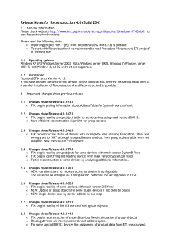
Explanation of the Calculation of the dr
Figure: Calculation of the dr
Calculation of the dr :
Take k − 1 sequential points i ⇒ k − 1 equations
P
The dr have to fulfill k−1
r=0 dr = 1 ⇒ 1 equation
Solve the k equations for the k unknowns.
CASA Seminar
WENO-Schemes & Applications
Reconstruction
WENO
Numerical Implementation & Results
Basics
Coefficients for Convex Combination
Coefficients ωr
We require the following properties of the coefficients:
If v(x) is smooth on Sr (i) we want
ωr ≈ dr
hence
ωr = O(1).
If v(x) has a discontinuity inside Sr (i) ωr should be
essentially 0, i.e.
ωr = O(∆x` ).
CASA Seminar
WENO-Schemes & Applications
Reconstruction
WENO
Numerical Implementation & Results
Basics
Coefficients for Convex Combination
Calculation of ωr
Combining these aspects we get
αr
ωr = Pk−1
s=0
αs
r = 0, . . . , k − 1
,
where αr is given by
αr =
dr
.
(ε + βr )2
with ε ∈ [10−5 , 10−7 ] (usually 10− 6). The βr are the so-called
“smooth indicators”.
CASA Seminar
WENO-Schemes & Applications
Reconstruction
WENO
Numerical Implementation & Results
Basics
Coefficients for Convex Combination
Smooth indicator βr
If v(x) is smooth in Sr (i) one wants
βr = O(∆x2 )
and for discontinuous v one obtains
βr = O(1).
One choice for βr which fulfills the requirements is
βr =
k−1 Z
X
l=1
xi+ 1
2
2l−1
∆x
xi− 1
∂ l pr (x)
∂xl
2
dx.
2
CASA Seminar
WENO-Schemes & Applications
Reconstruction
WENO
Numerical Implementation & Results
Basics
Coefficients for Convex Combination
WENO Procedure
(r)
1
Calculate the k reconstructed values vi+ 1 for each i.
2
Find the constants dr .
3
Find the smooth indicators βr .
4
Form the weights ωr .
5
The (2k − 1)-th order reconstruction is given by
2
vi+ 1 =
2
k−1
X
r=0
(r)
ωr vi+ 1 .
2
−
Note, that the values vi+ 1 are later denoted by vi+
1.
2
2
+
Additionally one can obtain the values vi−
1 for the cell i using
the same considerations.
CASA Seminar
2
WENO-Schemes & Applications
Reconstruction
WENO
Numerical Implementation & Results
Basics
Coefficients for Convex Combination
Comparison of the Reconstruction
Figure: Comparison of the fixed-stencil approx.(fixed r = 1) left and
the WENO(k = 3) right for ∆x = 0.02.
CASA Seminar
WENO-Schemes & Applications
Reconstruction
WENO
Numerical Implementation & Results
FVM
1D scalar FDM with WENO-Roe
1D scalar FDM with flux-splitting
Burger’s equation using FVM and WENO
CASA Seminar
WENO-Schemes & Applications
Reconstruction
WENO
Numerical Implementation & Results
FVM
1D scalar FDM with WENO-Roe
1D scalar FDM with flux-splitting
FDM approximation
We use a conservative approximation to the spatial derivative
1 ˆ
dui (t)
=−
fi+ 1 − ˆfi− 1 .
2
2
dt
∆x
ui (t) is the numerical approximation to the point value u(xi , t).
We want
1 ˆ
fi+ 1 − ˆfi− 1 = fx (u(xi , t)) + O(∆xk )
∀ i.
2
2
∆xi
This numerical flux is obtained by ENO or WENO
reconstruction using the setting
v
¯(x) = f(u(x, t)).
CASA Seminar
WENO-Schemes & Applications
Reconstruction
WENO
Numerical Implementation & Results
FVM
1D scalar FDM with WENO-Roe
1D scalar FDM with flux-splitting
Upwinding using the Roe speed
We have to define the Roe speed
ai+ 1 :=
¯
2
f(ui+1 ) − f(ui )
.
ui+1 − ui
−
+
Depending on the sign of the ¯ai+ 1 one uses vi+
for the
1 or v
i+ 1
2
numerical flux, i.e.
2
2
if ¯
ai+ 1 ≥ 0 one says that the wind blows from the left,
2
hence one uses v− 1 for the numerical flux ˆf 1 .
i+ 2
i+ 2
if ¯ai+ 1 < 0 one says that the wind blows from the right,
2
hence one uses v+ 1 for the numerical flux ˆf 1 .
i+ 2
CASA Seminar
i+ 2
WENO-Schemes & Applications
Reconstruction
WENO
Numerical Implementation & Results
FVM
1D scalar FDM with WENO-Roe
1D scalar FDM with flux-splitting
Burger’s equation using FDM and WENO-Roe
CASA Seminar
WENO-Schemes & Applications
Reconstruction
WENO
Numerical Implementation & Results
FVM
1D scalar FDM with WENO-Roe
1D scalar FDM with flux-splitting
Burger’s equation using FDM and WENO-Roe 2
CASA Seminar
WENO-Schemes & Applications
Reconstruction
WENO
Numerical Implementation & Results
FVM
1D scalar FDM with WENO-Roe
1D scalar FDM with flux-splitting
Flux-splitting
A more stable approach is to use a splitting of the flux, i.e.
f(u) = f + (u) + f − (u)
where
df + (u)
df − (u)
≥ 0 and
≤ 0.
du
du
hold. For example the Lax-Friedrich splitting:
1
f ± (u) = (f(u) ± αu)
2
where α is defined by
α = max |f 0 (u)|
u
CASA Seminar
WENO-Schemes & Applications
Reconstruction
WENO
Numerical Implementation & Results
FVM
1D scalar FDM with WENO-Roe
1D scalar FDM with flux-splitting
Flux splitting procedure
The numerical flux is then obtained by the following procedure:
1
Identify v
¯i = f + (u(xi )) and use ENO or WENO
−
reconstruction procedure to obtain the values vi+
1.
2
2
Set the positive numerical flux as
ˆf + 1 = v− 1 .
i+
i+
2
2
f − (u(xi ))
3
Identify v
¯i =
and use ENO or WENO
+
reconstruction procedure to obtain the values vi+
1.
4
Set the negative numerical flux as
ˆf − 1 = v+ 1 .
2
i+ 2
5
i+ 2
Form the numerical flux as
ˆf 1 = ˆf + 1 + ˆf − 1 .
i+
i+
i+
2
CASA Seminar
2
2
WENO-Schemes & Applications
Reconstruction
WENO
Numerical Implementation & Results
FVM
1D scalar FDM with WENO-Roe
1D scalar FDM with flux-splitting
Burger’s equation using FDM with flux-splitting
CASA Seminar
WENO-Schemes & Applications

Download Report